This document describes a MATLAB® tool for deriving and solving circuit equations symbolically. It is split up into several segments.
Before using the program you must first download it from GitHub and save it on your computer where MATLAB can access it. Note: you must have the symbolic toolbox to run this code. The example netlists described on this page are also on GitHub.
The code is provided as-is and there is no guarantee that it is without bugs. If you do find a bug, please contact me.
The code is written as a MATLAB script instead of a function because I thought it would make learning easier because it can be stepped through, and all of the variables created by the code appear in the workspace so users can examine and manipulate them. If you don't want all of the variables in your workspace, it is straightforward to add a line at the top to turn it into a function. If you don't want all the intermediate results printed, simply comment out the lines you don't want.
There is essentially no error checking, so if you enter a netlist that isn't correct the program will fail without explaining why.
Notational conventions:
The SCAM program cannot simply read a schematic diagram so we need to develop a method for representing a circuit textually. This can be done using a device called a netlist that defines the interconnection between circuit elements. If you have used SPICE (Simulation Program with Integrated Circuit Emphasis) this is a familiar concept. A good review is given by Jan Van Der Spiegel at the University of Pennsylvania. The process is easily demonstrated by example.
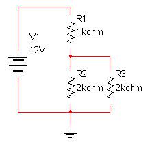
Let's use SCAM to analyze the circuit below:

We start by defining the nodes. The only restriction here is that the nodes must be labeled such that ground is node 0, and the other nodes are named consecutively starting at 1. The choice of which number to assign to which node is entirely arbitrary.
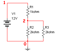
SCAM requires a text file with one line for each component in the circuit. This circuit has 4 components (3 resistors and 1voltage source), and will require 6 lines to define it. Each type of component has its own format for its corresponding lines in a file. These are shown below. The labels N1, N2, etc... correspond to the nodes in the circuit.
| Component Type | Symbol | SCAM Description |
| Resistor |  |
R1 N1 N2 1000
|
| Capacitor |  |
C1 N1 N2 1E-6
|
| Inductor | L1 N1 N2 1E-3
|
|
| Voltage Source |  |
V1 N1 N2 12
|
| Current Source |  |
I1 N1 N2 1
|
| Op Amp |  |
O1 N1 N2 N3
|
Define the current through the voltage source to give a final circuit diagram:
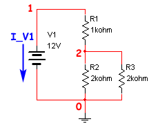
The netlist file is:
V1 1 0 12
R1 1 2 1000
R2 2 0 2000
R3 2 0 2000
Let's use the circuit we have been examining

We will create a text file containing the netlist:
V1 1 0 12
R1 1 2 1000
R2 2 0 2000
R3 2 0 2000
and save it in the directory seen by MATLAB. I edited such a file (using the MATLAB editor) and saved it in my SCAM directory as example1.cir. To run the program, assign the filename of the circuit to be analyzed to the variable fname, and then call the program. The output from the MATLAB window is shown below:
>> fname="example1.cir";
>> scam

Started -- please be patient.

Netlist:
V1 1 0 12
R1 1 2 1000
R2 2 0 2000
R3 2 0 2000

The A matrix:
[  1/R1,              -1/R1, 1]
[ -1/R1, 1/R1 + 1/R2 + 1/R3, 0]
[     1,                  0, 0]

The x matrix:
  v_1
  v_2
 I_V1

The z matrix:
  0
  0
 V1

The matrix equation:
            I_V1 + v_1/R1 - v_2/R1 == 0
 v_2*(1/R1 + 1/R2 + 1/R3) - v_1/R1 == 0
                              v_1 == V1

The solution:
                                       v_1 == V1
       v_2 == (R2*R3*V1)/(R1*R2 + R1*R3 + R2*R3)
 I_V1 == -(V1*(R2 + R3))/(R1*R2 + R1*R3 + R2*R3)

Elapsed time is 0.308426 seconds.
The netlist is displayed, followed by A, x and z matrices as well as the matrix equations written out. Finally the values of the unknow variables are displayed. Let's look at the value of v_2 (the voltage at node 2):
>> v_2
v_2 = (R2*R3*V1)/(R1*R2 + R1*R3 + R2*R3)
or I_V1 (the current through the voltage source)
>> I_V1
I_V1 = -(V1*(R2 + R3))/(R1*R2 + R1*R3 + R2*R3)
In addition to the unknowns, several other variables are created in the workspace (this is why the SCAM program is a script instead of a function). The important variables created, in addition to the unknowns, are a value corresponding to each of the elements. We can examine the value of any element, for example V1 or R2
>> V1
V1 =    12

>> R1
R1 =    1000
We can use these values to get numeric values for the unknowns:
>> eval(v_2)
ans =     6

>> eval(I_V1)
ans =   -0.0060
which shows that the voltage at node 2 is 6 volts, and the current through V1 is 6 mA (into the positive node).
What happens if we are interested in the current through R2 instead of just node voltages, from node 2 to node 0. We know that the current through R2 is just the voltage drop across R2, divided by the value of the resistance. We can do the solution either symbolically or numerically.
>> v_2/R2
ans = (R2*R3*V1)/(2000*(R1*R2 + R1*R3 + R2*R3))

>> eval(ans)
ans =    0.0030
The current through R1, from node 1 to node 2, is just the voltage across R1 divided by its value.
>> (v_1-v_2)/R1
ans = V1/1000 - (R2*R3*V1)/(1000*(R1*R2 + R1*R3 + R2*R3))

>> eval(ans)
ans =    0.0060
Other quantities can be similarly determined. For example the ratio of v_2 to V1:
>> v_2/V1
ans = (R2*R3*V1)/(12*(R1*R2 + R1*R3 + R2*R3))

>> eval ans
ans = (R2*R3*V1)/(12*(R1*R2 + R1*R3 + R2*R3))
The SCAM program also defines the A, x and z matrices from the MNA method.
>> A
A =
[  1/R1,              -1/R1, 1]
[ -1/R1, 1/R1 + 1/R2 + 1/R3, 0]
[     1,                  0, 0]

>> x
x =
  v_1
  v_2
 I_V1

>> z
z =
  0
  0
 V1
We can use these variables to recreate the circuit equations. To get the left side of the equations we just multiply A*X:
>> A*x
ans =
            I_V1 + v_1/R1 - v_2/R1
 v_2*(1/R1 + 1/R2 + 1/R3) - v_1/R1
                               v_1
or, in a slightly easier to read form:
>> pretty(A*x)
/             v_1   v_2      \
|      I_V1 + --- - ---      |
|              R1    R1      |
|                            |
|     /  1    1    1 \   v_1 |
| v_2 | -- + -- + -- | - --- |
|     \ R1   R2   R3 /    R1 |
|                            |
\             v_1            /
We can even get the Latex:
>> latex(A*x)
ans =
    '\left(\begin{array}{c} I_{\mathrm{V1}}+\frac{v_{1}}{R_{1}}-\frac{v_{2}}{R_{1}}\\ v_{2}\,\left(\frac{1}{R_{1}}+\frac{1}{R_{2}}+\frac{1}{R_{3}}\right)-\frac{v_{1}}{R_{1}}\\ v_{1} \end{array}\right)'
The left side of the equation is given by z:
>> z
z =
  0
  0
 V1
Using the information above, we can get any of the MNA equations. To get the equations for node 2, simply take the 2nd row of the right and left sides of the equations:
\[\begin{gathered} - \frac{{v\_1}}{{R1}} + \left( {\frac{1}{{R1}} + \frac{1}{{R2}} + \frac{1}{{R3}}} \right)v\_2 = 0 \hfill \\ or \hfill \\ \left( {\frac{{v\_2 - v\_1}}{{R1}}} \right) + \frac{{v\_2}}{{R2}} + \frac{{v\_2}}{{R3}} = 0 \hfill \\ \end{gathered} \]We can also apply the program to more complex circuits, such as the following (Example 3 from the MNA Examples page with values given to each component) (with nodes already labeled, and the currents through the voltage sources also labeled for clarity):
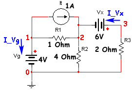
The netlist for this circuit is given by
Vg 1 0 4
Vx 3 2 6
R1 1 2 1
R2 2 0 4
R3 3 0 2
It 1 2 1
I entered this into a file and named it example4.cir. To analyze the circuit we proceed as before, by setting the fname variable, and starting the program:
>> fname='example4.cir';
>> scam

Started -- please be patient.

Netlist:
Vg 1 0 4
Vx 3 2 6
R1 1 2 1
R2 2 0 4
R3 3 0 2
It 1 2 1

The A matrix:
[  1/R1,       -1/R1,    0, 1,  0]
[ -1/R1, 1/R1 + 1/R2,    0, 0, -1]
[     0,           0, 1/R3, 0,  1]
[     1,           0,    0, 0,  0]
[     0,          -1,    1, 0,  0]

The x matrix:
  v_1
  v_2
  v_3
 I_Vg
 I_Vx

The z matrix:
 -It
  It
   0
  Vg
  Vx

The matrix equation:
           I_Vg + v_1/R1 - v_2/R1 == -It
 v_2*(1/R1 + 1/R2) - v_1/R1 - I_Vx == It
                      I_Vx + v_3/R3 == 0
                               v_1 == Vg
                         v_3 - v_2 == Vx

The solution:
                                                                      v_1 == Vg
             v_2 == (R2*R3*Vg - R1*R2*Vx + It*R1*R2*R3)/(R1*R2 + R1*R3 + R2*R3)
         v_3 == (R3*(R2*Vg + R1*Vx + R2*Vx + It*R1*R2))/(R1*R2 + R1*R3 + R2*R3)
 I_Vg == -(R2*Vg + R3*Vg + R2*Vx + It*R1*R2 + It*R1*R3)/(R1*R2 + R1*R3 + R2*R3)
            I_Vx == -(R2*Vg + R1*Vx + R2*Vx + It*R1*R2)/(R1*R2 + R1*R3 + R2*R3)

Elapsed time is 0.48674 seconds.
We can solve for the voltage at node 2 either symbolically or numerically:
>> v_2
v_2 = (R2*R3*Vg - R1*R2*Vx + It*R1*R2*R3)/(R1*R2 + R1*R3 + R2*R3)

>> eval(v_2)
ans =   1.1429
We can find the current through R1 (symbolically or numerically):
>> (v_1-v_2)/R1
ans =
Vg - (R2*R3*Vg - R1*R2*Vx + It*R1*R2*R3)/(R1*R2 + R1*R3 + R2*R3)
>> eval(ans)
ans =
    2.8571
We can find the MNA equation for node 2:
>> q=A*x==z
q =
           I_Vg + v_1/R1 - v_2/R1 == -It
 v_2*(1/R1 + 1/R2) - v_1/R1 - I_Vx == It
                      I_Vx + v_3/R3 == 0
                               v_1 == Vg
                         v_3 - v_2 == Vx

>> q(2)
ans = v_2*(1/R1 + 1/R2) - v_1/R1 - I_Vx == It

>> pretty(q(2))
    /  1    1 \   v_1
v_2 | -- + -- | - --- - I_Vx == It
    \ R1   R2 /    R1
or, in a cleaner format
\[ v_{2}\,\left(\frac{1}{R_{1}}+\frac{1}{R_{2}}\right)-\frac{v_{1}}{R_{1}}-I_{\mathrm{Vx}}=\mathrm{It} \]The next example shows an op-amp with 2 resistors in the standard inverting configuration along with its netlist (example5.cir).
| Circuit | Netlist | |
|
       Vin 3 0 Symbolic
       R1 1 3 Symbolic
       R2 2 1 Symbolic
OAmp 0 1 2 |
Since we don't have values for the components in the circuit, they are declared to be "Symbolic". We can now solve this circuit to determine the gain between Vin and node 2.
>> fname="example5.cir";
>> scam

Started -- please be patient.

Netlist:
Vin 3 0 Symbolic
R1 1 3 Symbolic
R2 2 1 Symbolic
OAmp 0 1 2

The A matrix:
[ 1/R1 + 1/R2, -1/R2, -1/R1, 0, 0]
[       -1/R2,  1/R2,     0, 0, 1]
[       -1/R1,     0,  1/R1, 1, 0]
[           0,     0,     1, 0, 0]
[          -1,     0,     0, 0, 0]

The x matrix:
    v_1
    v_2
    v_3
  I_Vin
 I_OAmp

The z matrix:
   0
   0
   0
 Vin
   0

The matrix equation:
 v_1*(1/R1 + 1/R2) - v_2/R2 - v_3/R1 == 0
            I_OAmp - v_1/R2 + v_2/R2 == 0
             I_Vin - v_1/R1 + v_3/R1 == 0
                               v_3 == Vin
                                -v_1 == 0

The solution:
            v_1 == 0
 v_2 == -(R2*Vin)/R1
          v_3 == Vin
    I_Vin == -Vin/R1
    I_OAmp == Vin/R1

Elapsed time is 0.423071 seconds.

>> v_2/Vin
ans = -R2/R1
Some notes on this circuit:
Often we would like to take our results and use them in MATLAB for other calculations. this is especially true when working with transfer functions. The example below shows how this can be accomplished. This circuit is from the MNA with Capacitors and Inductors page with values given to each component, with nodes already labeled, and the currents through the voltage sources also labeled for clarity. The netlist is called example6.cir.
| Circuit | Netlist | |
|
       Vin 3 0 Symbolic
       R2 3 2 1000
       R1 1 0 1000
       C1 1 0 1E-6
       C2 2 1 10E-6
L1 1 0 0.001 |
Now let's solve and get the transfer function symbolically
>> fname="example6.cir";
>> scam

Started -- please be patient.

Netlist:
Vin 3 0 Symbolic
R2 3 2 1000
R1 1 0 1000
C1 1 0 1E-6
C2 2 1 10E-6
L1 1 0 0.001

The A matrix:
[ C1*s + C2*s + 1/R1 + 1/(L1*s),       -C2*s,     0, 0]
[                         -C2*s, C2*s + 1/R2, -1/R2, 0]
[                             0,       -1/R2,  1/R2, 1]
[                             0,           0,     1, 0]

The x matrix:
   v_1
   v_2
   v_3
 I_Vin

The z matrix:
   0
   0
   0
 Vin

The matrix equation:
 v_1*(C1*s + C2*s + 1/R1 + 1/(L1*s)) - C2*s*v_2 == 0
          v_2*(C2*s + 1/R2) - v_3/R2 - C2*s*v_1 == 0
                        I_Vin - v_2/R2 + v_3/R2 == 0
                                          v_3 == Vin

The solution:
                               v_1 == (C2*L1*R1*Vin*s^2)/(R1 + L1*s + C1*L1*R1*s^2 + C2*L1*R1*s^2 + C2*L1*R2*s^2 + C2*R1*R2*s + C1*C2*L1*R1*R2*s^3)
  v_2 == (Vin*(R1 + L1*s + C1*L1*R1*s^2 + C2*L1*R1*s^2))/(R1 + L1*s + C1*L1*R1*s^2 + C2*L1*R1*s^2 + C2*L1*R2*s^2 + C2*R1*R2*s + C1*C2*L1*R1*R2*s^3)
                                                                                                                                         v_3 == Vin
 I_Vin == -(Vin*(C1*C2*L1*R1*s^3 + C2*L1*s^2 + C2*R1*s))/(R1 + L1*s + C1*L1*R1*s^2 + C2*L1*R1*s^2 + C2*L1*R2*s^2 + C2*R1*R2*s + C1*C2*L1*R1*R2*s^3)

Elapsed time is 0.380204 seconds.

>> H=v_2/Vin              %Find transfer function between input and node 2
H =
(R1 + L1*s + C1*L1*R1*s^2 + C2*L1*R1*s^2)/(R1 + L1*s + C1*L1*R1*s^2 + C2*L1*R1*s^2 + C2*L1*R2*s^2 + C2*R1*R2*s + C1*C2*L1*R1*R2*s^3)

>> H=collect(H)
H =
((C1*L1*R1 + C2*L1*R1)*s^2 + L1*s + R1)/(C1*C2*L1*R1*R2*s^3 + (C1*L1*R1 + C2*L1*R1 + C2*L1*R2)*s^2 + (L1 + C2*R1*R2)*s + R1)

>> pretty(H)           % Pretty print it.
                                             2
                      (C1 L1 R1 + C2 L1 R1) s  + L1 s + R1
--------------------------------------------------------------------------------
                3                                     2
C1 C2 L1 R1 R2 s  + (C1 L1 R1 + C2 L1 R1 + C2 L1 R2) s  + (L1 + C2 R1 R2) s + R1
We can also get a numerical transfer function
>> Hnumbers = eval(H)
Hnumbers =
((6493253913945763*s^2)/590295810358705651712 + s/1000 + 1000)/(s^3/100000000 + (3099053004383205*s^2)/147573952589676412928 + (10001*s)/1000 + 1000)
While this answer is correct, it is not in a very convenient form, and we can't do any actual simulation with it. However we can easily convert the expression to a MATLAB transfer function object. First we separate out the numerator and denominator, and then convert them to MATLAB polynomials.
>> Hnumbers = eval(H)
Hnumbers =
((6493253913945763*s^2)/590295810358705651712 + s/1000 + 1000)/(s^3/100000000 + (3099053004383205*s^2)/147573952589676412928 + (10001*s)/1000 + 1000)

>> [n,d]=numden(Hnumbers)
n =
2536427310135063671875*s^2 + 230584300921369395200000*s + 230584300921369395200000000000
d =
2305843009213693952*s^3 + 4842270319348757812500*s^2 + 2306073593514615321395200000*s + 230584300921369395200000000000

>> mySys=tf(sym2poly(n),sym2poly(d))
mySys =
         2.536e21 s^2 + 2.306e23 s + 2.306e29
  ---------------------------------------------------
  2.306e18 s^3 + 4.842e21 s^2 + 2.306e27 s + 2.306e29

Continuous-time transfer function.
The transfer function is still in an odd form (we'd like the highest powers of 's' in the denominator to have a coefficient of 1). Fortunately, MATLAB's "minreal()" function does this.
>> mySys=minreal(mySys)
mySys =
    1100 s^2 + 100000 s + 1e11
  ------------------------------
  s^3 + 2100 s^2 + 1e09 s + 1e11

Continuous-time transfer function.
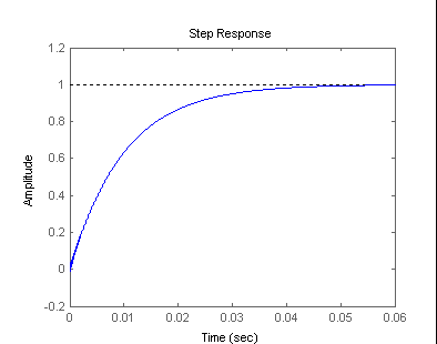
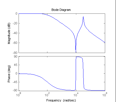
We are now free to perform any of the MATLAB function relating to polynomials. Shown below are a step response and a Bode plot.
| Step Response | Bode Plot |
| >> step(mySys) | >>bode(mySys) |
 |
 |
Now consider the case of finding the current through a wire. In particular, consider the previous circuit:
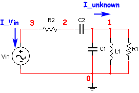
We would like to find the current shown. How do we do this. One way would be to find each current into and out of node 1 and solve for the unknown current. Another way is to introduce a voltage source of zero volts (i.e., a short circuit), and its concomitant node. The netlist is example7.cir.
| Circuit | Netlist | |
|
       Vin 3 0 Symbolic
       R2 3 2 1000
       R1 1 0 1000
       C1 4 0 1E-6
       C2 2 4 10E-6
       L1 1 0 0.001
Vsc 4 1 0 |
This voltage source has no effect on the circuit, but forces the computation of the current I_Vsc.
>> fname="example7.cir";
>> scam

Started -- please be patient.

Netlist:
Vin 3 0 Symbolic
R2 3 2 1000
R1 1 0 1000
C1 4 0 1E-6
C2 2 4 10E-6
L1 1 0 0.001
Vsc 4 1 0

The A matrix:
[ 1/R1 + 1/(L1*s),           0,     0,           0, 0, -1]
[               0, C2*s + 1/R2, -1/R2,       -C2*s, 0,  0]
[               0,       -1/R2,  1/R2,           0, 1,  0]
[               0,       -C2*s,     0, C1*s + C2*s, 0,  1]
[               0,           0,     1,           0, 0,  0]
[              -1,           0,     0,           1, 0,  0]

The x matrix:
   v_1
   v_2
   v_3
   v_4
 I_Vin
 I_Vsc

The z matrix:
   0
   0
   0
   0
 Vin
 Vsc

The matrix equation:
         v_1*(1/R1 + 1/(L1*s)) - I_Vsc == 0
 v_2*(C2*s + 1/R2) - v_3/R2 - C2*s*v_4 == 0
               I_Vin - v_2/R2 + v_3/R2 == 0
  I_Vsc + v_4*(C1*s + C2*s) - C2*s*v_2 == 0
                                 v_3 == Vin
                           v_4 - v_1 == Vsc

The solution:
            v_1 == -(C1*L1*R1*Vsc*s^2 - C2*L1*R1*Vin*s^2 + C2*L1*R1*Vsc*s^2 + C1*C2*L1*R1*R2*Vsc*s^3)/(R1 + L1*s + C1*L1*R1*s^2 + C2*L1*R1*s^2 + C2*L1*R2*s^2 + C2*R1*R2*s + C1*C2*L1*R1*R2*s^3)
 v_2 == (R1*Vin + L1*Vin*s + C2*R1*R2*Vsc*s + C1*L1*R1*Vin*s^2 + C2*L1*R1*Vin*s^2 + C2*L1*R2*Vsc*s^2)/(R1 + L1*s + C1*L1*R1*s^2 + C2*L1*R1*s^2 + C2*L1*R2*s^2 + C2*R1*R2*s + C1*C2*L1*R1*R2*s^3)
                                                                                                                                                                                      v_3 == Vin
                    v_4 == (R1*Vsc + L1*Vsc*s + C2*R1*R2*Vsc*s + C2*L1*R1*Vin*s^2 + C2*L1*R2*Vsc*s^2)/(R1 + L1*s + C1*L1*R1*s^2 + C2*L1*R1*s^2 + C2*L1*R2*s^2 + C2*R1*R2*s + C1*C2*L1*R1*R2*s^3)
                          I_Vin == -(C2*s*(R1*Vin - R1*Vsc + L1*Vin*s - L1*Vsc*s + C1*L1*R1*Vin*s^2))/(R1 + L1*s + C1*L1*R1*s^2 + C2*L1*R1*s^2 + C2*L1*R2*s^2 + C2*R1*R2*s + C1*C2*L1*R1*R2*s^3)
                                I_Vsc == -(s*(R1 + L1*s)*(C1*Vsc - C2*Vin + C2*Vsc + C1*C2*R2*Vsc*s))/(R1 + L1*s + C1*L1*R1*s^2 + C2*L1*R1*s^2 + C2*L1*R2*s^2 + C2*R1*R2*s + C1*C2*L1*R1*R2*s^3)

Elapsed time is 0.703828 seconds.
>> eval(I_Vsc)
ans =
(Vin*s*(s/1000 + 1000))/(100000*(s^3/100000000 + (21*s^2)/1000000 + (10001*s)/1000 + 1000))
>> simplify(ans)
ans =
(Vin*s*(s + 1000000))/(s^3 + 2100*s^2 + 1000100000*s + 100000000000)
>> pretty(ans)
            Vin s (s + 1000000)
------------------------------------------
 3         2
s  + 2100 s  + 1000100000 s + 100000000000
This is the end of my description of SCAM. We have come a long way from some simple circuit theory, to a description of Modified Nodal Analysis (along with an algorithm for applying MNA - including reactive elements and op-amps), to this page describing a MATLAB tool that performs MNA on a circuit, given a netlist.
I hope you find SCAM to be a useful tool. Please contact me with any comments or errors.
If you are interested in how dependent sources can be handled, check out the next page.