
Contents
Consider the system shown. In this diagram m=3 kg, b=0.6 N-s/m, and k=1.5 N/m. The position of the mass is x(t), and x(t)=0 at equilibrium. The initial velocity (at t=0-) is -2 m/s, and the initial position is x(0-)=0 m. The input is a force on the mass, fa(t), of 6 Newtons to the right for t≥0.
Note: the vertical axis has units of Newtons for the input, fa(t), and units of meters for the output, x(t).
The question at hand is: how can we calculate the position of m? To do this we must first develop a mathematical model of the system. We can draw a free body diagram

From this we can write the system differential equation.

We must now solve this equation.
Let us solve the equation

with

so

An easy way to do this is simply to:
Step 1) Take the Laplace Transform of the differential equation:
Using the differentiation property of the Laplace Transform, and the Laplace Transform of the unit step function we get the Laplace Transform pair,

Putting in the initial condition yields the algebraic equation:

Step 2) Solve the resulting algebraic equation
We solve for our output, X(s):
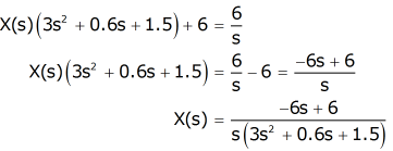
It is useful to give the highest order term in the numerator a coefficient of one, so we multiply the numerator and denominator by 1/3..

Step 3) Take the inverse Laplace Transform using Partial Fraction Expansion
We can perform the partial fraction expansion by hand, or use a tool like MatLab. If we do it by hand, we get:

Cross multiply to find coefficients

Equate terms with like powers of s

From the bottom equation we get A=4, which yields (from the other two equations) B=-4 and C=-2.8. Thus, our equation becomes

To get forms in the table, we must complete the square

We can then look this up in the Laplace Transform Table (see entry for generic decaying oscillatory (alternate))
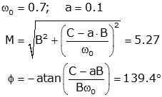 (Note)
atan is the arctangent (tan-1) function. The atan function can give incorrect results (typically the function is written so that the result is always in quadrants I or IV). To ensure accuracy, use a function that corrects for this. In most programming languages the function is atan2. Also be careful about using degrees and radians as appropriate.

We could also solve this problem using MatLab to perform the partial fraction expansion
>> [r,p,k]=residue([-2 2],[1 0.2 0.5 0])
r =
  -2.0000 + 1.7143i
  -2.0000 - 1.7143i
   4.0000

p =
  -0.1000 + 0.7000i
  -0.1000 - 0.7000i
        0

k =    []

>> M=2*abs(r(1))
M =
    5.2683

>> phi=angle(r(1))*180/pi
phi =
  139.3987
From these results (and using "Method 1 - a more general technique" from the inverse Laplace Transform page) we get the same solution.

So the final solution is

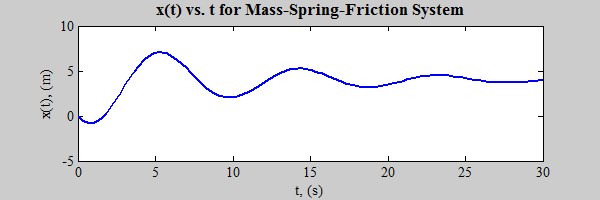
This can be verified by plotting with MatLab. It is apparent that the analytic solution is identical to that of the simulation (above).
>> t=linspace(0,30);
>> x=4+5.27*exp(-0.1*t).*cos(0.7*t+139.4*pi/180);  %(with phi in radians)
>> plot(t,x)
>> title('x(t) vs. t for Mass-Spring-Friction System'); xlabel('t, (s)');  ylabel('x(t), (m)');
While the method described above (find system model, convert to Laplace, solve, perform inverse Laplace) is straightforward and is, in fact, often the simplest way to to solve a problem, there is another common method. It is possible to split up the solution of the problem into two parts, the zero input solution, and the zero state solution. The zero input solution is the response of the system to the initial conditions, with the input set to zero. The zero state solution is the response of the system to the input, with initial conditions set to zero. The complete response is simply the sum of the zero input and zero state response.
The question naturally arises: why split a single problem into two separate problems? There are several reasons: the two problems are each easier to solve; the effects of the initial conditions are separated from those due to the inputs; if the solution is to be solved with several different initial conditions (or inputs), only part of the problem needs to be solved again.
We will now resolve the original problem (from above) using zero input and zero state solutions. The problem is restated here for convenience.

To solve the zero input problem, we set the input to zero and change x to xzi to indicate that it is now the zero input solution.

Take the Laplace Transform, apply the initial conditions and solve for Xzi(s).

To get this into a form that in the table (see entry for generic decaying oscillatory) we need only complete the square:

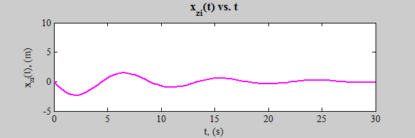
We can plot this with MatLab. Note: that the variable "t" was defined previously.
>> xzi=-2.86*exp(-0.1*t).*sin(0.7*t);
>> plot(t,xzi,'m')
>> title('x_{zi}(t) vs. t'); xlabel('t, (s)');  ylabel('x_{zi}(t), (m)'); axis([0 30 -5 10]);
To solve the zero state problem, we set the initial conditions to zero and change x to xzs and proceed as before.
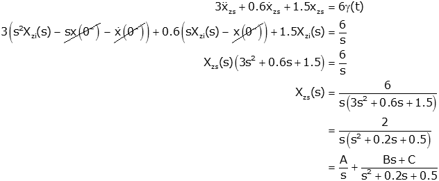
Find A, B, and C by cross multiplication followed by equating like powers of s:
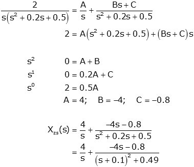
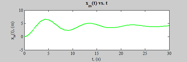
We look these terms up in the table (see entry for generic decaying oscillatory (alternate)) and plot with Matlab

>> xzs=4+4.04*exp(-0.1*t).*cos(0.7*t+171.9*pi/180);
>> plot(t,xzs,'g')
>> title('x_{zs}(t) vs. t'); xlabel('t, (s)');  ylabel('x_{zs}(t), (m)'); axis([0 30 -5 10]);
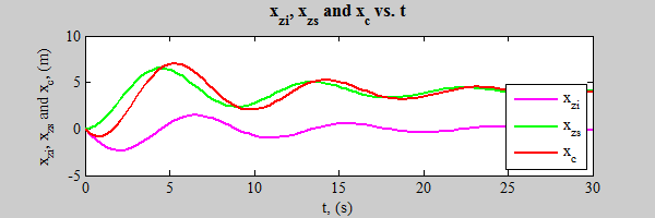
The complete solution is simply the sum of the zero input and zero state response - all three are plotted below (xzi and xzs were calculated previously):

>> xc=xzi+xzs;
>> plot(t,xzi,'m',t,xzs,'g',t,xc,'r');
>> legend('x_{zi}','x_{zs}','x_c','Location','se')
>> title('x_{zi}, x_{zs} and x_c vs. t');  xlabel('t, (s)');
>> ylabel('x_{zi}, x_{zs} and x_c, (m)')
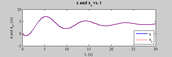
To show that this is the same as obtained previously, we plot both results (i.e., the response from the first (simplistic) method, and the complete response using zero state and zero input). Note, the variable "x" was defined previously.
>> plot(t,x,'b',t,xc,'r:');
>> legend('x','x_c','Location','se')
>> title('x and x_c vs. t');  xlabel('t, (s)'); ylabel('x and x_c, (m)')
The following four examples show how the zero input / zero state solution can simplify the solution of differential equations as the input and/or initial conditions change.
Solve the differential equation

with

Zero input solution
To find the zero input solution, take the Laplace Transform of the input with f(t)=0 and solve for Xzi(s).

Perform a partial fraction expansion and inverse transform.

Note: in these examples, the calculations of the partial fraction expansions will not be shown, and all functions of time are implicitly zero for t<0.
Zero State Solution
To find the zero state solution, take the Laplace Transform of the input with initial conditions=0 and solve for Xzs(s).
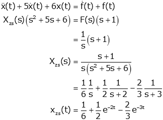
Complete Solution
The complete solutions is simply the sum of the zero state and zero input solution
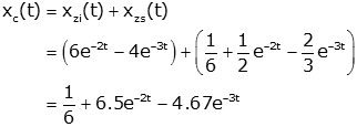
Solve the differential equation

with

Zero input solution
To find the zero input solution, take the Laplace Transform of the input with f(t)=0 and solve for Xzi(s).
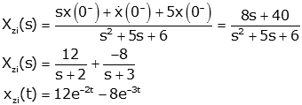
Note: since the initial condition was doubled, the zero input response was doubled. This would not have been as easy with the "simple" method introduced at the beginning of this page.
Zero State Solution
The input is the same as in Example 1a, so we don't need to solve it again.

Complete Solution
The complete solutions is simply the sum of the zero state and zero input solution

Solve the differential equation

with

Zero input solution
The initial conditions are the same as in Example 1a, so we don't need to solve it again.

Zero State Solution
To find the zero state solution, take the Laplace Transform of the input with initial conditions=0 and solve for Xzs(s).
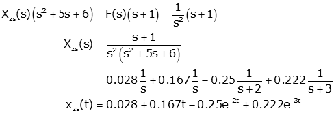
Complete Solution
The complete solutions is simply the sum of the zero state and zero input solution

Solve the differential equation

with

Zero input solution
The initial conditions are the same as in Example 1b, so we don't need to solve it again.

Zero State Solution
The input is the same as in Example 1c, so we don't need to solve it again.

Complete Solution
The complete solutions is simply the sum of the zero state and zero input solution

The power of the zero input / zero state solution is shown by the last example in which no extra work needed to be done to get the solution.
The transient response of a system can be found by splitting a problem into two parts.
The complete response is simply the sum of the zero input and zero state solutions.
This section is not yet finished, but it is not a critically important topic.