
Contents
To productively use the Laplace Transform, we need to be able to transform functions from the time domain to the Laplace domain. We can do this by applying the definition of the Laplace Transform

but this quickly becomes tedious. Our goal is to avoid having to evaluate the integral by finding the Laplace Transform of many useful functions and compiling them in a table. Thereafter the Laplace Transform of functions can almost always be looked by using the tables without any need to integrate. A table of Laplace Transform of functions is available here.
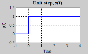
The unit step function is defined as

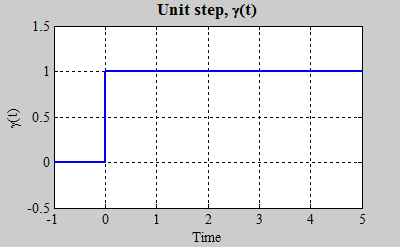
Some notes about this function:
To find the Laplace Transform, we apply the definition.
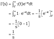
so

Careful inspection of the evaluation of the integral performed above:

reveals a problem. The evaluation of the upper limit of the integral only goes to zero if the real part of the complex variable "s" is positive (so e-st→0 as s→∞). In this case we say that the "region of convergence" of the Laplace Transform is the right half of the s-plane (since s is a complex number, the right half of the plane corresponds to the real part of s being positive). As long as the functions we are working with have at least part of their region of convergence in common (which will be true in the types of problems we consider), the region of convergence holds no particular interest for us. Since the region of convergence will not play a part in any of the problems we will solve, it is not considered further.
The unit impulse is discussed elsewhere, but to review. The impulse function is everywhere but at t=0, where it is infinitely large. The area of the impulse function is one. The impulse function is drawn as an arrow whose height is equal to its area.

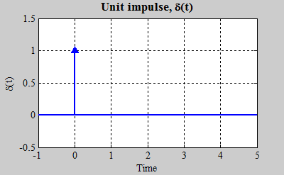
To find the Laplace Transform, we apply the definition

Now we apply the sifting property of the impulse. Since the impulse is 0 everywhere but t=0, we can change the upper limit of the integral to 0+.

Since e-st is continuous at t=0, that is the same as saying it is constant from t=0- to t=0+. So we can replace e-st by its value evaluated at t=0.

So the Laplace Transform of the unit impulse is just one. Therefore the impulse function, which is difficult to handle in the time domain, becomes easy to handle in the Laplace domain. It will turn out that the unit impulse will be important to much of what we do.
Consider the causal (i.e., defined only for t>0) exponential:

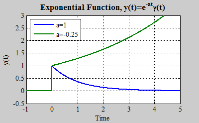
Several notes about this function:
To find the Laplace Transform, we apply the definition

Since γ(t) is equal to one for all positive t, we can remove it from the integral
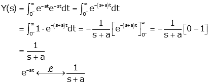 (Note)
Convergence: As with the step function, the region of convergence is limited for the exponential. The integral only converges if the real part of (s+a) is positive so the function decays as t→∞. In other words, the region of convergence is a half-plane in s where the Real(s)>-Real(a).
Note that multiplication by the function γ(t) is implicit on the left hand side of the last equation. This is how we will commonly write our functions.
Note that if a=0, we get a step function and Y(s)=1/s.

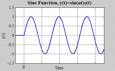
As before, start with the definition of the Laplace transform

Here it becomes useful to use Euler's identity for the sine

so

But we've already done this integral (the exponential function, above)

Let's put this over a common denominator
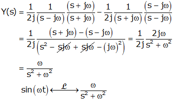

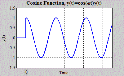
The cosine can be found in much the same way, but using Euler's identity for the cosine.

Note that if ω=0, we get a step function and Y(s)=1/s.
The decaying sine or cosine is likewise handled in the same way. Consider, first, the decaying sine wave.

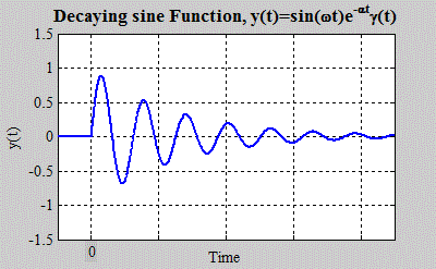

The rest of the derivation follows that of the sine function (i.e., put over a common denominator, and solve)

A similar procedure can be followed for the decaying cosine

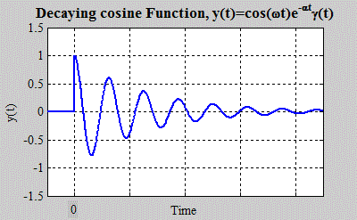

So far (with the exception of the impulse), all the functions have been closely related to the exponential. It is also possible to find the Laplace Transform of other functions. For example, the ramp function:

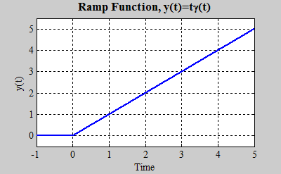
We start as before

Integration by parts is useful at this point
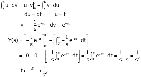
It is often quite easy to find the Laplace Transform of functions not in the table, by expressing them as a sum of functions in the table that are scaled and/or delayed. To understand this we need to use two Laplace Transform properties that are derived on the next page. We need the linearity property

and the time delay property

Find the Laplace Transform of the function shown:
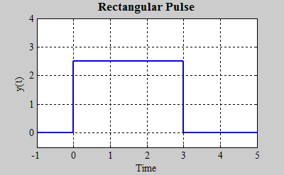
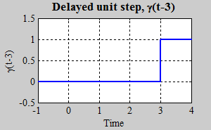
We can compose this function in terms of two other functions
Solution:
We know the Laplace Transform of both of these
functions

Let's see if we can use this information to find the Laplace Transform of the rectangular pulse. We can form the original rectangular pulse function from the step and the delayed step in two ways
| Method 1 | Method 2 |
 |
 |
The first method doesn't help us, because we have no property of the Laplace Transform the lets us deal with multiplied functions in the time domain. However, the second method can be used because it represents y(t) as the sum of functions, so we can use the linearity property. So we get

The addition of the two functions is shown graphically below

and y(t)=2.5·z(t)
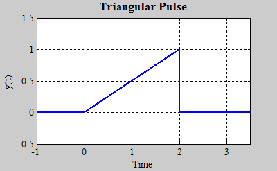
Find the Laplace Transform of the function shown:
Solution:
We need to figure out how to represent the
function as the sum of functions with which we are familiar.
For this function, we need only ramps and steps; we apply a ramp function at
each change in slope of y(t), and apply a step at each discontinuity.
Functionally we want:

so

Graphically this is shown as:
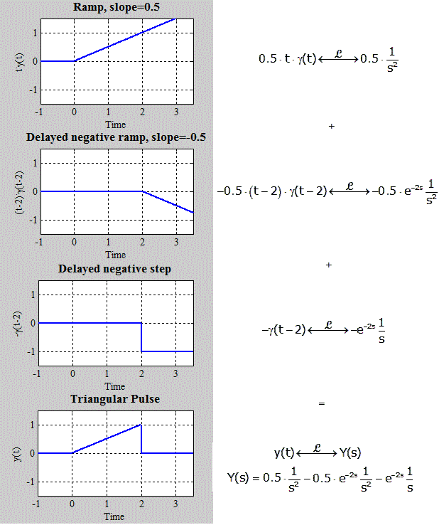
It may seem like it would be easier to define the function as a ramp (0.5·t) multiplied by a rectangular pulse (γ(t)-γ(t-1))

and this does, in fact, yield the correct function. However if we do this we end up with the product of two functions that are in the table separately

However, these two functions have different time delays and we have no way to deal with products of functions. That is why, when choosing the basic functions that make up the composite function, only addition is allowed. (Note)
It is OK to have multiplication of a function by the unit step as long as both functions have the same time delay. That is because the role of the unit step in that case is solely to make sure that the function is zero before it starts.
Find the Laplace Transform of the function shown:
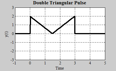
Solution:
This function is more complicated than the
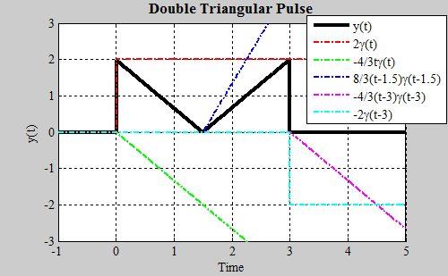
last, but we can still create it as a sum of ramps and steps; we apply a ramp
function at each change in slope of y(t), and apply a step at each discontinuity.

The constituent functions are shown in the plot below. If you add them up, you get the original function (shown in black).
Find the Laplace Transform of the function shown:
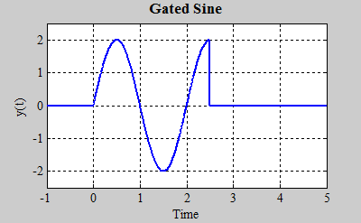
Solution:
This function is a little different than the
previous in that it involves more than ramps and steps. The most obvious
way to represent this function is as a sine wave multiplied by a rectangular
pulse. But recall that we can't use generally use multiplication of functions (we have
no multiplication property), only addition (by use of the linearity
property). So the question becomes: what functions can we add to
create the given function?
After a little thought it becomes apparent that we can take a sine wave starting at t=0, and subtract off a cosine beginning at t=2.5.

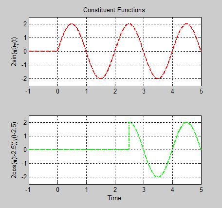
When composing a complex function from elementary functions, it is important to only use addition. If you create a function by adding two functions, its Laplace Transform is simply the sum of the Laplace Transform of the two function. If you create a function by multiplying two functions in time, there is no easy way to find the Laplace Transform of the resulting function.
A table of Laplace Transform of functions is available here.