
As systems become more complex, representing them with differential equations or transfer functions becomes cumbersome. This is even more true if the system has multiple inputs and outputs. This document introduces the state space method which largely alleviates this problem. The state space representation of a system replaces an nth order differential equation with a single first order matrix differential equation. The state space representation of a system is given by two equations :

Note: Bold face characters denote a vector or matrix.The variable x is more commonly used in textbooks and other references than is the variable q when state variables are discussed. The variable q will be used here since we will often use x to represent position.
The first equation is called the state equation, the second equation is called the output equation. For an nth order system (i.e., it can be represented by an nth order differential equation) with r inputs and m outputs the size of each of the matrices is as follows:
Note several features:
For systems with a single input and single output (i.e., most of the systems we will consider) these variables become (with r=1 and m=1):

where
Advantages of this representation include:
Consider an 4th order system represented by a single 4th order differential equation with input x and output z.

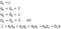
We can define 4 new variables, q1 through q4.
but

We can now rewrite the 4th order differential equation as 4 first order equations

This is compactly written in state space format as
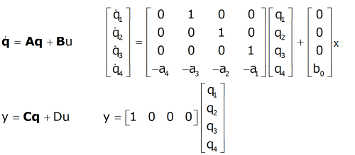
with

For this problem a state space representation was easy to find. In many cases (e.g., if there are derivatives on the right side of the differential equation) this problem can be much more difficult. Such cases are explained in the discussion of transformations between system representations.
Another important point is that the state space representation is not unique. As a simple example we could simply reorder the variables from the example above (the new state variables are labeled qnew). This results in a new state space representation
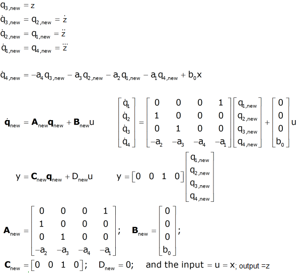
In the previous case careful examination of the original and modified state space system reveals that they represent the same system. However we can make entirely new state variables by forming linear combination of the original state variables in which this equality is not obvious. Consider the state variable qnew defined as follows:

In this case the new state space variables are given by (the details of how these matrices are determined are not important for this discussion. They are given here if you are interested):
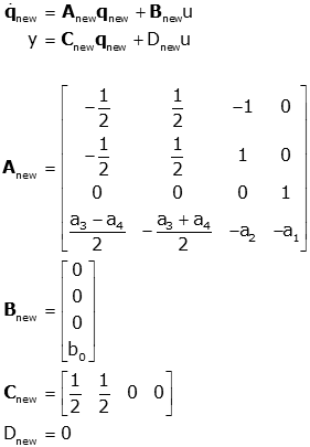
This new state space system is quite different from the original one, and it is not at all obvious that they represent the same system. (It can be shown that the systems are identical by transforming the state space representation to a transfer function. Techniques for doing so are discussed elsewhere.)
A nth order linear physical system can be represented using a state space approach as a single first order matrix differential equation:

The first equation is called the state equation and it has a first order derivative of the state variable(s) on the left, and the state variable(s) and input(s), multiplied by matrices, on the right. The second equation is called the output equation and it has the output on the left and the state variable(s) and input(s), multiplied by matrices, on the right. No other terms are allowed in the equation. In these equations:
For a single input, single output system (the case that interests us the most):

The state space representation is not unique; many (actually an infinite number) of state space systems can be used to represent any linear physical system.
Another, powerful, way to develop a state space model is directly from the free body diagrams. If you choose as your state variables those quantities that determine the energy in the system, a state space system is often easy to derive. For example, in a mechanical system you would choose extension of springs (potential energy, ½kx²) and the velocity of masses (kinetic energy, ½mv²); for electrical systems choose voltage across capacitors, ½Ce² (e=voltage)) and current through inductors (½Li²). This is best illustrated by several examples, two rotating and one electrical.
Derive a state space model for the system shown. The input is fa and the output is z.
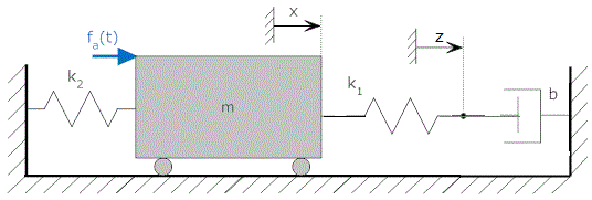
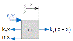
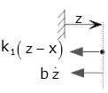
We can write free body equations for the system at x and at y.
| Freebody Diagram | Equation |
 |
 |
 |
 |
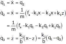
There are three energy storage elements, so we expect three state equations. The energy storage elements are the spring, k2, the mass, m, and the spring, k1. Therefore we choose as our state variables x (the energy in spring k2 is ½k2x²), the velocity at x (the energy in the mass m is ½mv², where v is the first derivative of x), and y (the energy in spring k1 is ½k1(z-x)² , so we could pick z-x as a state variable, but we'll just use z (since x is already a state variable; recall that the choice of state variables is not unique). Our state variables become:

Now we want equations for their derivatives. The equations of motion from the free body diagrams yield
or
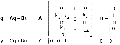
with the input u=fa, and the output y=z.
This technique does not always easily yield a set of state equations (read about some examples here). In some cases it is easier to develop a transfer function model and convert this to a state space model. Transfer functions are discussed elsewhere.
The energy variables for rotating systems are potential energy stored in springs (½Krθ²) and kinetic energy stored in inertial elements (½Jω²).
Derive a state space model for the system shown. The input is τa and the output is θ1.
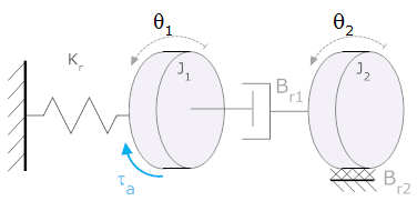
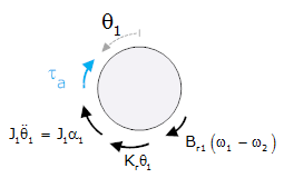
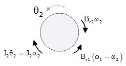
We can write free body equations for the system at θ1 and θ2
| Freebody Diagram | Equation |
|
 |
 |
 |
There are three energy storage elements, so we expect three state equations. Energy is stored as potential energy in the spring (½Krθ1²) and kinetic energy in the two flywheels (½J1α1², ½J2α2²). Our state variable equations become:

Now we want equations for their derivatives. The equations of motion from the free body diagrams yield
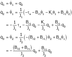
or
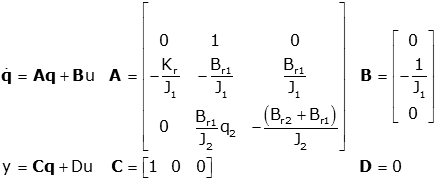
with the input u=τa, and the output y=θ1.
To develop a state space system for an electrical system, try choosing the voltage across capacitors, and current through inductors as state variables. Recall that

so if we can write equations for the voltage across an inductor, it becomes a state equation when we divide by the inductance (i.e., if we have an equation for einductor and divide by L, it becomes an equation for diinductor/dt which is one of our state variables). Likewise if we can write an equation for the current through the capacitor and divide by the capacitance it becomes a state equation for ecapacitor. This is best illustrated by an example.
Derive a state space model for the system shown. The input is ia and the output is e2.
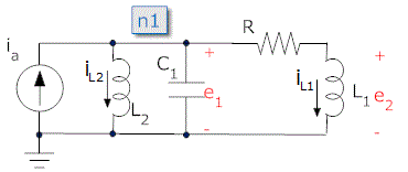
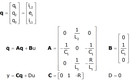
There are three energy storage elements, so we expect three state equations. Try choosing i1, i2 and e1 as state variables. Now we want equations for their derivatives. The voltage across the inductor L2 is e1 (which is one of our state variables)

so our first state variable equation is

If we sum currents into the node labeled n1 we get

This equation has our input (ia) and two state variable (iL2 and iL1) and the current through the capacitor. So from this we can get our second state equation

Our third, and final, state equation we get by writing an equation for the voltage across L1 (which is e2) in terms of our other state variables

We also need an output equation:

So our state space representation becomes
This technique does not always easily yield a set of state equations. In some cases it is easier to develop a transfer function model and convert this to a state space model. Transfer functions are discussed elsewhere.
There are several cases when it is not so straightforward to develop a state space model from a system diagram. Some of these are discussed here.
The state space representation of a system is a common and extremely powerful method of representing a system mathematically. This page only discusses how to develop the state space representation, the solution of state space problems are discussed elsewhere.
Since state space is equivalent to the other representations, there must be a way to transform from one representation to another. These methods are discussed here.