
Contents
Two of the most powerful (and common) ways to represent systems are the transfer function form and the state space form. This page describes how to transform a transfer function to a state space representation, and vice versa. Converting from state space form to a transfer function is straightforward because the transfer function form is unique. Converting from transfer function to state space is more involved, largely because there are many state space forms to describe a system.
Consider the state space system:

Now, take the Laplace Transform (with zero initial conditions since we are finding a transfer function):

We want to solve for the ratio of Y(s) to U(s), so we need so remove Q(s) from the output equation. We start by solving the state equation for Q(s)

The matrix Φ(s) is called the state transition matrix. Now we put this into the output equation

Now we can solve for the transfer function:

Note that although there are many state space representations of a given system, all of those representations will result in the same transfer function (i.e., the transfer function of a system is unique; the state space representation is not).
Find the transfer function of the system with state space representation
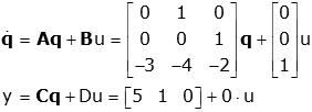
First find (sI-A) and the Φ=(sI-A)-1 (note: this calculation is not obvious. Details are here). Rules for inverting a 3x3 matrix are here.
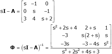
Now we can find the transfer function

To make this task easier, MatLab has a command (ss2tf) for converting from state space to transfer function.
>> % First define state space system
>> A=[0 1 0; 0 0 1; -3 -4 -2];
>> B=[0; 0; 1];
>> C=[5 1 0];
>> [n,d]=ss2tf(A,B,C,D)

n =
         0         0    1.0000    5.0000
d =
    1.0000    2.0000    4.0000    3.0000

>> mySys_tf=tf(n,d)
Transfer function:
       s + 5
----------------------
 s^3 + 2 s^2 + 4 s + 3
Find the transfer function of the system with state space representation
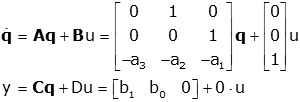
First find (sI-A) and the Φ=(sI-A)-1 (note: this calculation is not obvious. Details are here).
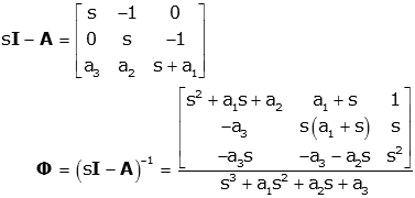
Now we can find the transfer function

Given a state space representation of a system

the transfer function is give by

and the characteristic equation (i.e., the denominator of the transfer function) is

Recall that state space models of systems are not unique; a system has many state space representations. Therefore we will develop a few methods for creating state space models of systems.
Before we look at procedures for converting from a transfer function to a state space model of a system, let's first examine going from a differential equation to state space. We'll do this first with a simple system, then move to a more complex system that will demonstrate the usefulness of a standard technique.
First we start with an example demonstrating a simple way of converting from a single differential equation to state space, followed by a conversion from transfer function to state space.
Consider the differential equation with no derivatives on the right hand side. We'll use a third order equation, thought it generalizes to nth order in the obvious way.

For such systems (no derivatives of the input) we can choose as our n state variables the variable y and its first n-1 derivatives (in this case the first two derivatives)

Taking the derivatives we can develop our state space model
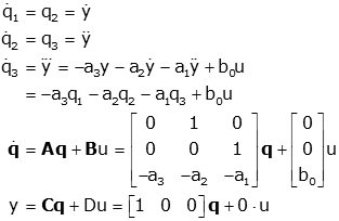
Note: For an nth order system the matrices generalize in the obvious way (A has ones above the main diagonal and the differential equation constants for the last row, B is all zeros with b0 in the bottom row, C is zero except for the leftmost element which is one, and D is zero)
Consider the transfer function with a constant numerator (note: this is the same system as in the preceding example). We'll use a third order equation, thought it generalizes to nth order in the obvious way.

For such systems (no derivatives of the input) we can choose as our n state variables the variable y and its first n-1 derivatives (in this case the first two derivatives)

Taking the derivatives we can develop our state space model (which is exactly the same as when we started from the differential equation)
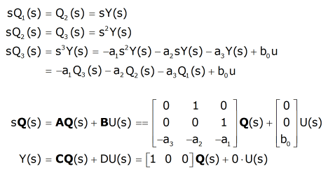
Note: For an nth order system the matrices generalize in the obvious way (A has ones above the main diagonal and the coefficients of the denominator polynomial for the last row, B is all zeros with b0 (the numerator coefficient) in the bottom row, C is zero except for the leftmost element which is one, and D is zero)
If we try this method on a slightly more complicated system, we find that it initially fails (though we can succeed with a little cleverness).
Consider the differential equation with a single derivative on the right hand side.

We can try the same method as before:
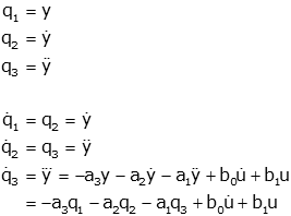
The method has failed because there is a derivative of the input on the
right hand, and that is not allowed in a state space model.
Fortunately we can solve our problem by revising our choice of state variables.

Now when we take the derivatives we get:

The second and third equations are not correct, because ÿ is not one of the state variables. However we can make use of the fact:

The second state variable equation then becomes

In the third state variable equation we have successfully removed the derivative of the input from the right side of the third equation, and we can get rid of the ÿ term using the same substitution we used for the second state variable.
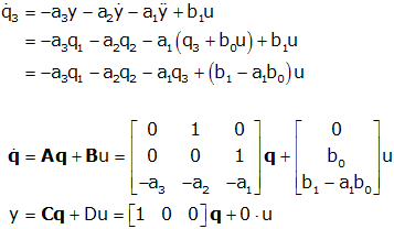
The process described in the previous example can be generalized to systems with higher order input derivatives but unfortunately gets increasingly difficult as the order of the derivative increases. When the order of derivatives is equal on both sides, the process becomes much more difficult (and the variable "D" is no longer equal to zero). Clearly more straightforward techniques are necessary. Two are outlined below, one generates a state space method known as the "controllable canonical form" and the other generates the "observable canonical form (the meaning of these terms derives from Control Theory but are not important to us).
Probably the most straightforward method for converting from the transfer function of a system to a state space model is to generate a model in "controllable canonical form." This term comes from Control Theory but its exact meaning is not important to us. To see how this method of generating a state space model works, consider the third order differential transfer function:

We start by multiplying by Z(s)/Z(s) and then solving for Y(s) and U(s) in terms of Z(s). We also convert back to a differential equation.

We can now choose z and its first two derivatives as our state variables

Now we just need to form the output

From these results we can easily form the state space model:
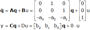
In this case, the order of the numerator of the transfer function was less than that of the denominator. If they are equal, the process is somewhat more complex. A result that works in all cases is given below; the details are here. For a general nth order transfer function:

the controllable canonical state space model form is

For a general nth order transfer function:

the controllable canonical state space model form is

Another commonly used state variable form is the "observable canonical form." This term comes from Control Theory but its exact meaning is not important to us. To understand how this method works consider a third order system with transfer function:

We can convert this to a differential equation and solve for the highest order derivative of y:

Now we integrate twice (the reason for this will be apparent soon), and collect terms according to order of the integral:

Choose the output as our first state variable

Looking at the right hand side of the differential equation we note that y=q1 and we call the two integral terms q2:

so

This is our first state variable equation.
Now let's examine q2 and its derivative:

Again we note that y=q1 and we call the integral terms q3:

so

This is our second state variable equation.
Now let's examine q3 and its derivative:

This is our third, and last, state variable equation.
Our state space model now becomes:
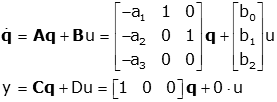
In this case, the order of the numerator of the transfer function was less than that of the denominator. If they are equal, the process is somewhat more complex. A result that works in all cases is given below; the details are here. For a general nth order transfer function:

the observable canonical state space model form is
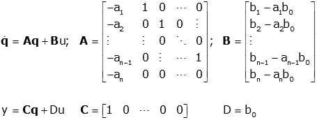
For a general nth order transfer function:

the observable canonical state space model form is

There are many other forms that are possible. For example MATLAB uses a
variant of the controllability canonical form in its "ss2tf"
function.
© Copyright 2005 to 2019 Erik Cheever This page may be freely used for educational purposes.
Erik Cheever Department of Engineering Swarthmore College