
Contents
Before starting this section make sure you understand how to create a state space representation of a system.
Zero input and zero state solutions of a system can be found if a state space representation of the system is known. Before solving an example, we first develop a generalized technique for finding the zero input and zero state solutions of a problem. This is followed by several examples.
Recall that a state space system is defined by the equations

where q is the state vector, A is the state matrix, B is the input matrix, u is the input, C is the output matrix, D is the direct transition (or feedthrough) matrix, and y is the output. In general we will have a single input and single output so u(t), y(t) and D defined as scalars. The techniques generalize in obvious ways to systems with multiple inputs and multiple outputs.
Before we consider the solution of a problem, we will first introduce the state transition matrix and discuss some of its properties. The state transition matrix is an important part of both the zero input and the zero state solutions of systems represented in state space. The state transition matrix in the Laplace Domain, Φ(s), is defined as:

where I is the identity matrix. The time domain state transition matrix, φ(t), is simply the inverse Laplace Transform of Φ(s).
Find
Φ(s) and φ(t) if

Solution:
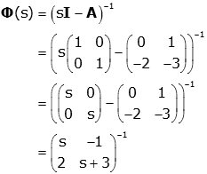
The inverse of a 2×2 matrix is given here.
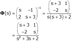
To find φ(t) we must take the inverse Laplace Transform of every term in the matrix
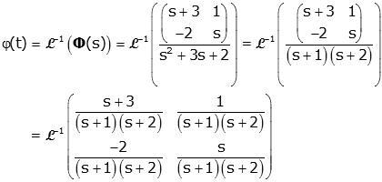
We now must perform a partial fraction expansion of each term, and solve
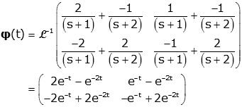
Solution via MatLab
MatLab can be used to find the zero input
response of a state space system:
Let us now develop a method for finding the zero input solution to a system defined in state space. The system is defined as

The zero input problem is given by:

with a known set of initial conditions, q(0-).
We solve for q(t) by first taking the Laplace Transform and solving for Q(s)
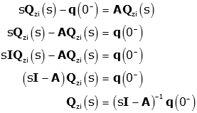
But, (sI-A)-1=Φ(s), i.e., the state transition matrix. So

Since q(0-) is a constant multiplier the inverse Laplace Transform is simply

The solution for y(t) is found in a straightforward way from the output equation

Find the response for the system defined by:

with

and

Solution:
The zero input problem was
solved previously

with the state transition matrix given by

For the given A matrix, Φ(s) and φ(t) were calculated previously (above)
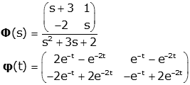
So
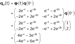
and
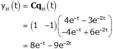
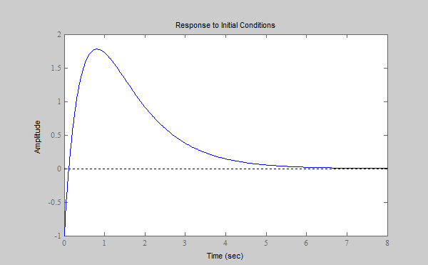
Solution via Matlab
This problem can also be solve
with MatLab
A=[0 1; -2 -3];             %Define Matrices
B=[0; 1;];  C=[1 -1];  D=0;
mySys=ss(A,B,C,D);          %Define State Space system
q0=[1; 2;];                 %Define initial conditions
initial(mySys,q0);          %Plot zero input solution
Given a state space system:

The zero input response is given by


where Φ(s) is the state transition matrix:

There is an alternate, more intuitive, derivation of the state transition matrix. This derivation is made in analogy with that of a scalar first order differential equation. The scalar and matrix equations are shown below, side-by-side.
| Description | Scalar Equation | Matrix Equation |
| Define the problem (a 1st order differential equation) |
 |
  |
| Write solution in terms of initial conditions and |
 |
 |
| (Taylor expansion of exponential) |  |
 |
Examining the third row of the table we see that we have introduced a matrix exponential that is exactly analogous to the scalar exponential, and we have used this matrix exponential in the solution of our first order matrix differential equation:

Comparing this to our solution in terms of the state transition matrix

we see that

Write a closed form expression for eAt if
 .
.
Solution:
Since

and we know (from above) that for the A matrix specified that

then

It is perhaps surprising that the series form of the matrix exponential

yields such a compact closed form solution, but this makes it possible to evaluate eAt (and φ(t)) precisely and efficiently.
From the matrix exponential definition of the state transition matrix we can derive several properties.
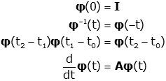
Finding the zero state response of a system given a state space representation is a bit more complicated. In the Laplace Domain the response is found by first finding the transfer function of the system. (A description of the transformation from state space representation to transfer function is given elsewhere).
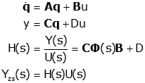
In the time domain, this last equation (multiplication in the Laplace domain), is just a convolution (the asterisk (*) denotes convolution):

Note: this last equation assumes a single input system. For multi-input systems the u(t) term must stay to the right of B.
Find the zero input solution (qzi(t) and yzi(t)) for the system defined by:

with

and

Solution:
First we need to find the
transfer function from the state space representation

We found Φ(s); earlier.

so
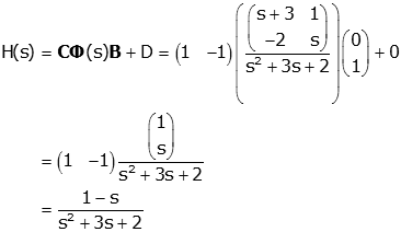
(we can check this with MatLab)
>> mySys=ss([0 1; -2 -3], [0; 1], [1 -1], 0);	% Define system in state space
>> [n,d]=tfdata(mySys,'v')   		% Get numerator and denominator
n =
         0   -1.0000    1.0000
d =
     1     3     2
We also know that

so

The partial fraction expansion can be done by hand or with Matlab. The Matlab solution is shown.
>> [r,p,k]=residue([1 -1],[1 3 2 0 0])	% Perform partial fraction expansion
r =
    0.7500
   -2.0000
   -1.2500
    0.5000
p =
    -2
    -1
     0
     0
k =  []

Find the response for the system defined by:

with

and

Solution:
The zero input problem was
solved previously

The zero state problem was also solved previously

The complete response is simply the sum of the two

Solution via Matlab
A numerical
solution can be found with Matlab
t=linspace(0,10);           %Define time vector
A=[0 1; -2 -3];             %Define Matrices
B=[0; 1;];  C=[1 -1];  D=0;
mySys=ss(A,B,C,D);          %Define State Space system

u=t;                        %Define input
q0=[1; 2;];                 %Define initial conditions

yzi=initial(mySys,q0,t);    %Find zero input response
yzs=lsim(mySys,u,t);        %Find zero state response
yc=yzi+yzs;                 %Find complete response
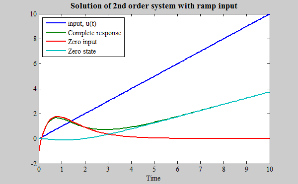
Note that the complete response converges to the zero state response at long times as the zero input response decays to zero.
The system shown is a simplified model of a part of a suspension system of a wheel on a car or motorcyle. The mass, m, represents the weight of the vehicle supported by the wheel, and the spring and dashpot represent the suspension system. For our purposes let m=500 kg, k=3000 N/m, b=2500 N-m/s.
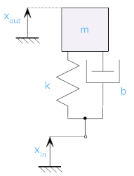
Find the output if the system starts at rest (the velocity is zero) but xout(0-)=0.05 and xin(t)=0.1·γ(t).
Solution:
We must first develop a state space model. Techniques for doing so are discussed elsewhere. We will start from the system transfer function (derived on the previous page):

We can transform this to Observable Canonic form as

From the output equation we see that

From the top row of the state variable equation we see that:

or

Zero State Solution:
We start by finding the state
transition matrix. This could be done by hand, we'll use Matlab's
symbolic toolbox:
>> syms s
>> A=[-5 1; -6 0];
>> Phi=inv(s*eye(2)-A)
Phi =
[  s/(s^2 + 5*s + 6),       1/(s^2 + 5*s + 6)]
[ -6/(s^2 + 5*s + 6), (s + 5)/(s^2 + 5*s + 6)]

The zero input solution is

with

We again turn to Matlab to find Yzi(s)
>> C=[1 0];
>> q0=[0.05; 0.25];
>> Yzi=C*Phi*q0
Yzi =
 s/(20*(s^2 + 5*s + 6)) + 1/(4*(s^2 + 5*s + 6))

>> pretty(simple(Yzi))
        s + 5
  -----------------
       2
  20 (s  + 5 s + 6)
At this point we could perform a partial fraction expansion, but we will let Matlab do the work
>> [r,p,k]=residue([1 5],20*[1 5 6])
r =
   -0.1000
    0.1500
p =
   -3.0000
   -2.0000
k =     []
So we get

As expected this agrees with the solution obtained using the transfer function (done on previous page).
Zero State Solution:
We start by finding the
transfer function, which was derived at the start of the problem.

(Note, if we didn't already know the transfer function we could always use the relationship H(s)=CΦ(s)B+D.)
Rather than solving this again, we refer to the solution on the previous page.

Complete Solution:
The complete response is simply the sum of the zero input and zero stat response.

© Copyright 2005 to 2019 Erik Cheever This page may be freely used for educational purposes.
Erik Cheever Department of Engineering Swarthmore College