Review of Arrays, Vectors and Matrices

This page is meant to be a brief review of the notation and elementary operations associated with arrays.  For our purposes vectors will be one dimensional arrays, and matrices will be two dimensional arrays.  If you feel comfortable with arrays, feel free to skip it.

Contents

• Vectors
• Matrices
• Matrix Operations
• Important Matrices
• Solution of Linear Algebraic Equations

Vectors

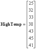
Vectors are an efficient notational method for representing lists of numbers. A typical vector might represent the high temperature every day for a week. Such a vector would have seven elements and could be written as a row vector (a single row),

or as a column vector (a single column),

Note, that I will use bold letters when referring to the entire vector (or matrix). In both cases above, the HighTemp vector has seven elements, representing Sunday through Saturday. To access the individual elements in the array we use an index. For example, the temperature Sunday would be accessed as HighTemp(1), and is equal to 25. Likewise HighTemp(4)=38 is Wednesday's high temperature.

Matrices

A matrix (singular of matrices) is for our purposes a series of numbers listed in two dimensions. As an example, consider high temperatures collected over a 28 day period (4 weeks). We could write the matrix as a single list 28 elements long, or as a collection of numbers (a matrix) that has 4 rows and 7 columns.

Now we need two indices to represent the numbers, one for the row, and one for the column. For example the high temperature during the 2^nd week, on the 3^rd day of that week,  is HighTemp(2,3) and is equal to 45. Note that the index for the row comes first.

In general a matrix consisting of m×n elements can be arranged in m rows and n columns, yielding an m×n (read m by n) matrix, which we'll call A. 

The symbol a_ij represents the number in the i^th row and the j^th column.  Note that a vector is the special case of a matrix, where there is only one row or column - In this case, the second subscript is dropped.

Matrix operations

For the ensuing discussion assume we have three matrices

Equality

Two matrices are equal if they are the same size, and corresponding elements are equal. For example, A=B, but A≠C.

Addition

Two matrices can be added if they are the same size. Their sum is given by a third matrix whose elements are the sum of the corresponding elements being added.of the two arrays.  In other words, if D=A+C then d_ij=a_ij+c_ij.

Note that matrix addition is commutative, X+Y=X+Y.

Transpose of a matrix

We could also write the matrix with rows and columns interchanged. This is referred to as taking the "transpose" of the matrix.  We'll denote the transpose with a single quote, '.  In other words, if D=A', then d_ij=a_ji. 

A matrix need not be square in order to take its transpose.  The transpose of a column vector is a row vector, and vice versa.

Multiplication by a scalar

A matrix can be multiplied by a scalar (a scalar is a single number) by multiplying each element of the array by that number. For example if D=2·A, then d_ij=2·a_ij.

Multiplication of two matrices

Two matrices, A and C can be multiplied together in the order A·C if and only if the number of columns in A equals the number of rows in C. If D=A·C, then d_ij is the element obtained by multiplying the row vector represented by the i^th row of A by the column vector represented by the j^th column of C. For arrays A and C with n columns and rows, respectively, we get:

For example, if D=A·C, using the matrices given previously

Note that in general A·C≠C·A. In this case

Expressed another way in words.  if D=A^.C, then the element in D located at row i and column j is given by the sum of the product of the elements in row i of A and the elements in column j of C.

Multiplication of two vectors

A row vector can be multiplied by a column vector, in that order, if and only if the have the same number of elements. If

,   then 

Determinant of a matrix

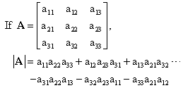
The determinant of a square matrix A is a scalar defined by

where C_ik is referred to as the cofactor of a_ik, and

where M_ik is the minor of a_ik.  M_ik is the determinant of the matrix that remains of A after the i^th row and j^th column are deleted.  In general it can be computationally very difficult to calculate determinants.  If the matrix has more than 3 rows and columns, you should use a computer or calculator to help you.  For 2×2 or 3×3 matrices there is are shortcuts (that don't work for larger matrices).

This is simply the product of the terms identified by the blue arrow (down and to the right) minus the product of the red arrow (up and to the right).

A similar rule applies to the 3×3 matrix (but not larger matrices).  The only complication is that the arrows wrap around the matrix from the right side to the left.

Important Matrices

Identitity Matrix

The identity matrix is a square matrix that has ones along the main diagonal and zeros elsewhere.  The 2×2 identity matrix is shown below.

The identity matrix has the special property that A·I=I·A=A.

Inverse Matrix

If the matrix A has an inverse G, we write G=A^-1, and G·A=A·G=I.  Note that some matrices don't have inverses.

You can check for yourself that A·A^-1=I.

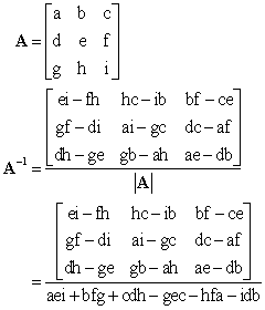
The inverse can be calculated as follows

where

and C_ik is the cofactor of a_ij. In general the inverse of a matrix is computationally very difficult to calculate.  If the matrix is greater than 2×2, use a calculator or a software package such as MatLab.  For a 2×2 matrix the inverse may be written as:

  For a 3×3 matrix the inverse may be written as:

Solution of Linear Systems of Algebraic Equations

Consider a linear system of algebraic equations with n equations and n unknowns:

In these equations, a_ij and b_i are constants, and the unknowns are x_i.  We can rewrite the equations as:

where

We can find all the unknowns in the vector x by doing a few simple matrix manipulations.  If we premultiply both sides of the matrix equation by the inverse of the A matrix we get:

which is our solution.

Note:  This discussion has assumed that all the equations are independent, i.e. that you can't form one of the equations from combinations of other equations.

>> A=[2 3 -1;-1 2 3;0 1 2]
A =
 2   3  -1
-1   2   3
 0   1   2

	
>> b=[-1 9 5]'
b =
-1
9
5

>> x=inv(A)*b
x =
-1
1
2

References