Convolution is a very powerful technique that can be used to calculate the zero state response (i.e., the response to an input when the system has zero initial conditions) of a system to an arbitrary input by using the impulse response of a system. It uses the power of linearity and superposition. To understand the power that this technique gives, consider the system described by the differential equation:
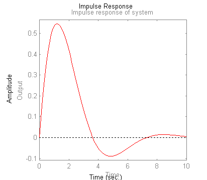
\[\ddot y\left( t \right) + \dot y\left( t \right) + y\left( t \right) = f\left( t \right)\]where y(t) is the output, and f(t) is the input. The impulse response of this system, h(t), can be shown to be equal to
$h\left( t \right) = \sqrt {\frac{4}{3}} {e^{ - 0.5t}}\sin \left( {\sqrt {\frac{3}{4}} t} \right),\quad t \geqslant 0\quad$ (from Laplace Transform Table)
The impulse response is shown graphically below.

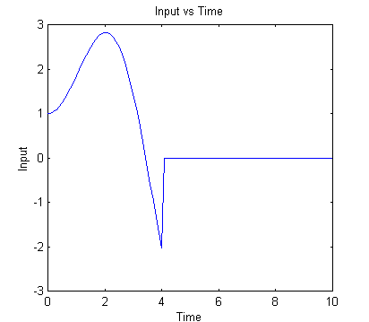
You know how to find the output y(t) if the input f(t) is a well defined input such as a step, impulse or sinusoid. Convolution allows you to determine the response to more complex inputs like the one shown below. In fact, you can use convolution to find the output for any input, if you know the impulse response. This gives incredible power.
There are several ways to understand how convolution works. First convolution will be developed in an approximate form as the sum of impulse responses. This presentation is useful for an intuitive understanding of the convolution process. After the approximate form is developed, the exact analytic form of convolution is given. You can also link to an example of the convolution integral in action, and to a less physical (more mathematical) derivation.
(the Matlab script, Convolution.m, was used to create all of the graphs in this section).
To understand how convolution works, we represent the continuous function shown above by a discrete function, as shown below, where we take a sample of the input every 0.8 seconds.
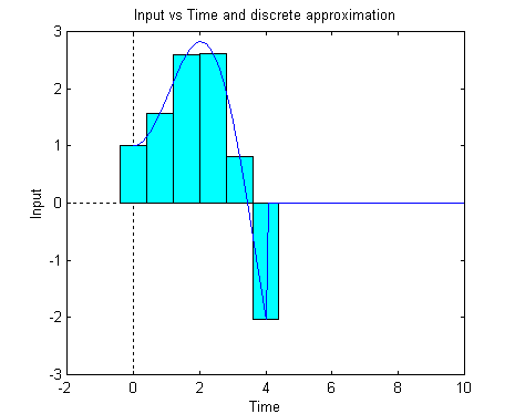
The approximation can be taken a step further by replacing each rectangular block by an impulse as shown below. The area of each impulse is the same as the area of the corresponding rectangular block. (Since the width of the block was 0.8, each impulse falls slightly below the function).
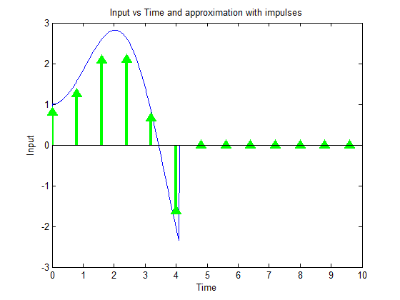
The superposition theorem states that the response of the system to the string of impulses is just the sum of the response to the individual impulses. The response of the system to the individual impulses is shown below.
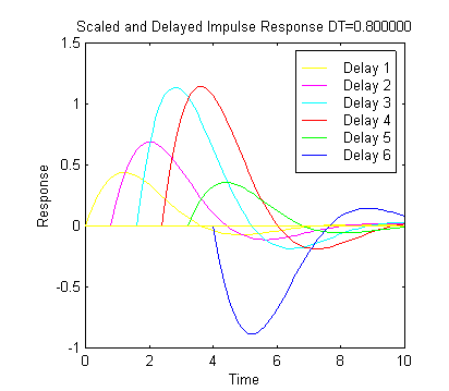
Lets look carefully at this graph and note the following:


This equation merely states that the output is equal to the sum of the responses from the individual impulses. Another (more mathematical) derivation of the convolution integral is given here.
The summed response is shown in the graph below, along with the individual responses.
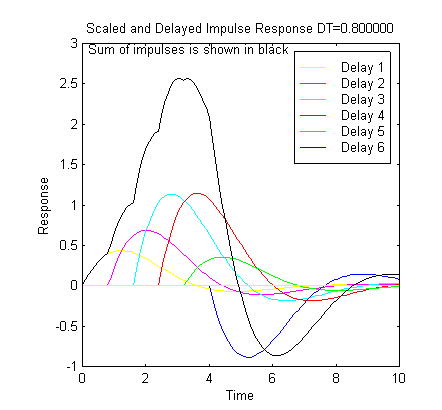
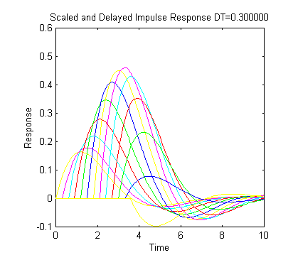
Obviously if you decrease the accuracy of the approximation should improve. The graph below shows the impulse responses if we let ΔT=0.3 seconds (instead of 0.8 seconds as shown above). Note that the individual responses are smaller, since the area of each impulse is smaller.
The graph below shows our approximate response, for ΔT=0.8 and ΔT=0.3, along with the exact response (the "exact" response is actually a numerical approximation, as calculated by Matlab).
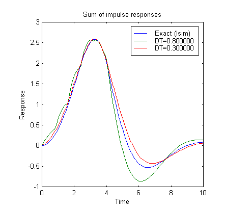
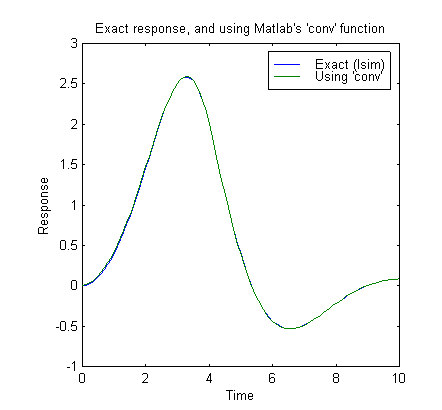
The graph below shows the "exact" response along with the response calculated using Matlab "conv" (convolve) function. Type "help conv" at the Matlab prompt to see how it works. Examine the script, convolution.m, which generated all these graphs for an example of how to use the function.
Hopefully this background gives you some physical insight into how convolution can be used to find the response of the system to an arbitrary input.
Convolution can be used to calculate the zero state response (i.e., the response to an input when the system has zero initial conditions) of a system to an arbitrary input by using the impulse response of a system. Given a system impulse response, h(t), and the input, f(t), the output, y(t) is the convolution of h(t) and f(t):

If h(t)=0 for t<0 and f(t)=0 for t<0 we can change the limits of integration such that:

To visualize the convolution we start from the definition:
\[y\left( t \right) = \int_{ - \infty }^{ + \infty } {f\left( \lambda \right)h\left( {t - \lambda } \right)d\lambda } \]or equivalently
\[y\left( t \right) = \int_0^t {f\left( \lambda \right)h\left( {t - \lambda } \right)d\lambda } \]if h(t)=0, t<0 and f(t)=0, t<0.
Consider the system discussed previously with the impulse response described by:
\[h\left( t \right) = \sqrt {\frac{4}{3}} {e^{ - 0.5t}}\sin \left( {\sqrt {\frac{3}{4}} t} \right),\quad t \geqslant 0\]as shown below
.gif)
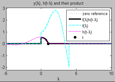
To find the response of the system, y(t), to an input, f(t), at t=1 sec we need to evaluate the integral
\[y\left( t \right) = \int_0^t {f\left( \lambda \right)h\left( {t - \lambda } \right)d\lambda } \]with t=1. To visualize this process consider the product f(λ)h(t-λ). A plot of f(λ) yields the input. A plot of h(t-λ) yields a time-reversed version of the impulse response with a time delay of t (1 second in this case). These are shown below along with the product of the two functions (solid black line). The function h(t-λ) is plotted in magenta and doesn't look much like the function above -- but note the different vertical scales.
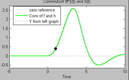
The next graph shows the result of the integration for all time, with a black dot at t=1.
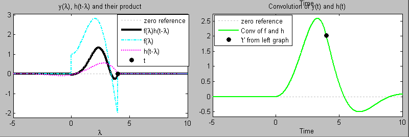
As t is increased further the function h(t-λ) shifts to the right. The multiplication and integration can be evaluated for each value of t to yield the system response y(t). The graphs below are similar to the ones above, except that t=4.
To see an animation of this shifting, multiplying and integrating process, click here.
Using the convolution integral it is possible to calculate the output, y(t), of any linear system given only the input, f(t), and the impulse response, h(t). However, this integration is often difficult, so we won't often do it explicitly. Later you will learn a technique that vastly simplifies the convolution process.
To see some more animations of convolutions, click here.
This page has given a description of the convolution process, but has not actually gone through the mathematical procedures needed to analytically evaluate the convolution integral when the input function has a piecewise definition. This process is described on another page. Click here to go to that page.
The MatLab code that generated the animations is available here.