


Several root locus examples are provided. Click on the transfer function to get to an explanation of how the root locus would be drawn by hand. The page also lets you enter your own transfer functions.
| Examples (Click on Transfer Function) | ||||
|---|---|---|---|---|
 |
 |
 |
 |
 |
The root locus is obviously a very powerful technique for design and analysis of control systems, but it must be used with some care, and results obtained with it should always be checked. To show potential pitfalls of this method, consider the two systems G1(s) and G2(s).
| G1(s) | G2(s) |
 |
 |
If we control these systems with a simple proportional controller, as shown,

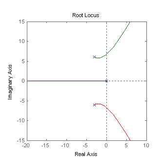
we can examine the root locus of each of them.
| Root Locus with G1(s) | Root Locus with G2(s) |
 |
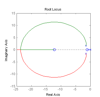 |
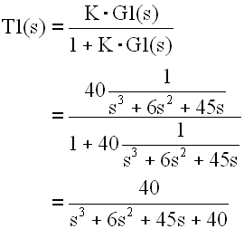
The two root loci are clearly very different, but it turns out (because of the way that I chose the systems) that if we choose K=40, we get two closed loop systems with identical characteristic equations.
| Closed loop system with G1(s) | Closed loop system with G2(s) |
 |
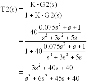 |
The roots of the characteristic equations are at s=-1 and s=-2.5±j5.8 (i.e., the roots of the characteristic equation s3+6s2+45s+40), so we might expect the behavior of the systems to be similar. Since the pole at s=-1 is closer to the origin, we would expect it to dominate somewhat, giving the system behavior similar to a first order system with a time constant of 1 second, and a settling time of 4 seconds. However, if we plot the two responses, we get something quite different.
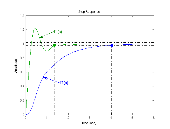
T1(s) resembles (somewhat) a first order system, and has no overshoot, and its settling time is almost exactly 4 seconds, as predicted. However, T2(s) behaves very differently, it is much faster and more oscillatory than expected. How can we explain this?
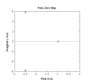
If we look more closely at T1(s) and T2(s), we can understand what happened. In particular, lets look at pole-zero plots of both closed loop transfer functions.
| Pole-Zero Plot of T1(s) | Pole-Zero Plot of T2(s) |
 |
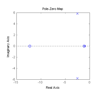 |
T1(s) has poles at s=-1 and s=-2.5±j5.8, and no zeros. T2(s) has poles at s=-1 and s=-2.5±j5.8 and zeros at -12.2 and -1.1. The zero at s=-1.1 is almost directly on top of the pole at s=-1, and so largely negates its effect. The closed loop system, T2(s), therefore behaves very much like a second order system with s=-2.5±j5.8 (ωn=6.3 rad/sec, and ζ=0.4).
The lesson here is that while the poles of a system (the roots of the denominator polynomial) are very important in determining the behavior of a system, the zeros of the system (the roots of the numerator polynomial) can also be important. After performing a root-locus design, it is critical to go back and test the closed loop system to ensure that it behaves as expected.