Contents
Eigenvalue/Eigenvector analysis is useful for a wide variety of differential equations. This page describes how it can be used in the study of vibration problems for a simple lumped parameter systems by considering a very simple system in detail. The next page describes gives a physical interpretation of the results and considers more complicated system.
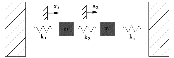
Consider the system shown below with 2 masses and 3 springs. The masses are constrained to move only in the horizontal direction (they can't move up an down):

We can draws the free body diagram for this system:
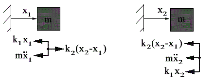
From this, we can get the equations of motion:
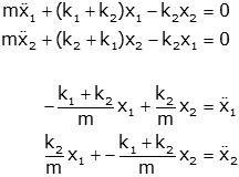
We can rearrange these into a matrix form (and use α and β for notational convenience).
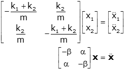

Now we proceed by assuming the form of solution (just as with differential equations). In this case, since there is no damping, we choose a purely oscillatory solution.

so
This is obviously just an eigenvalue problem. 

We can solve for the eigenvalues by finding the characteristic equation (note the "+" sign in the determinant rather than the "-" sign, because of the opposite signs of λ and ω2).
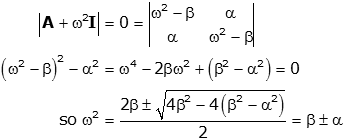
To make the notation easier we will now consider the specific case where k1=k2=m=1 so

Now we can also find the eigenvectors. For the first eigenvector:
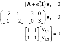
which clearly has the solution:

So we'll choose the first eigenvector (which can be multiplied by an arbitrary constant).

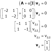
For the second eigenvector:
We can come up with a general form for the equations of motion for the two-mass system. The general solution is

Note that each frequency is used twice, because our solution was for the square of the frequency, which has two solutions (positive and negative). We will use initial condition to solve for the unknown coefficients, just like we did with differential equations. For a real response, the quantities c1 and c2 must be complex conjugates of each other, as are c3 and c4. The equation can then be re-written (the ordering of the γ coefficients becomes clear in a few steps):

We can use initial conditions to solve for the unknowns

Now let's consider the case when the initial condition on velocity is zero, and there is an arbitrary initial condition on position (this is the case we'll most often use):

Using the zero condition on initial velocity, we can write

which leads to the set of equations

Since we know that the frequencies are not equal to zero, we know the only solution is

Therefore, if the initial velocities are zero, only the cosine terms are needed and a general form for the solution simplifies to:

(Now the choice of the ordering of the γ coefficients is clear; this equation has γ1 and γ2 instead of γ1 and γ3)
We can find the coefficients γ1 and γ2 from the initial conditions.

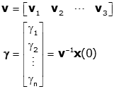
This yields a 2×2 set of equations that can be solved in a number of ways. Not surprisingly, the easiest way when using a computer is to formulate it as a matrix equation and solve. Start by forming a 2x2 matrix v whose columns are the eigenvectors of the problem

The equation for the initial conditions then becomes


The coefficient γ1 and γ2 are then easily found as the inverse of v multiplied by x(0)

Consider the case when k1=k2=m=1, as before, with initial conditions on the masses of

Assuming a solution of

we know that

We can write this as a set of two equations in two unknowns.

so

Thus the equations of motion is given by

or

Note: The two unknowns can also be solved for using only matrix manipulations by starting with the initial conditions and re-writing:

Now it is a simple task to find γ1 and γ2. This is the method used in the MatLab code shown below.
>> A=[-2 1;1 -2];       %Matrix determined by equations of motion.
>> [v,d]=eig(A)         %Find Eigenvalues and vectors.  The eigenvectors are the columns of "v," the eigenvectors are
                        %the diagonal elements of "d"
 v =
   0.7071  0.7071
  -0.7071  0.7071
 d =
  -3.0000  0
   0      -1.0000

>> x0=[1 0]'             %Initial conditions
 x0 =
   1
   0

>> gamma=inv(v)*x0	%Find unknown coefficients
 gamma =
   0.7071
   0.7071
%Define Array from equations of motion.
A=[-2 1;1 -2];            %2 masses
[v,d]=eig(A);             %Find Eigenvalues and vectors.
omega=sqrt(diag(-d));     %Get frequencies
x0=[1 0]'                 %Initial condition
gam=inv(v)*x0             %Find unknown coefficients


%nxn array with coefficients of gamma along the diagonal
g=diag(gam);
t=0:0.2:20;               %1xM Time vector (for plotting)
                          % cos(omega*t) is an nxM array with
                          %       cos(w1*t),...,cos(wn*t) in rows
x=v*g*cos(omega*t);       %Calculate output

% Display pertinent information about the system
disp('A matrix'); disp(A)
disp('Eigenvalues'); disp(diag(d)')
disp('Eigenvectors (each column is an eigenvector)'); disp(v)
disp(['Frequencies, omega=' sprintf('%4.2f, ',omega)]);
disp(['Initial Conditions, x(0)=' sprintf('%4.2f, ',x0)]);
disp(['Unknown coefficients, gamma=' sprintf('%4.2f, ',gam)]);

%This next code does some string manipulation to make
%legends for the plots, no calculations. It is not necessary
%to understand this code to understand the graphs;
N=size(A,1);
outLeg='';
modLeg='';
for i=1:N,
outLeg=strvcat(outLeg, strcat('Out_',int2str(i)));
mstr=sprintf('Mode_%d',i);
modLeg=strvcat(modLeg, mstr);
end

%Plot the output trajectories
subplot(2,1,1);
plot(t,x)
xlabel('Time'); ylabel('Output');
title(['Output vs. time, x_i(0)=' sprintf('%4.2f, ',x0) ...
' \gamma_i=' sprintf('%4.2f, ',gam)]);
legend(outLeg);

%Plot the mode shapes
subplot(2,1,2)
plot(v,':');
xlabel('Elements'); ylabel('Mode amplitude');
title(['Mode shapes, \omega=' sprintf('%4.2f, ',omega)]);
axis([0.5 N*1.5 -1 1]);
set(gca,'XTick',[1:N]);
legend(modLeg);
hold on
stem(v);
hold off

%Arrays for various numbers of masses.
A=[-2 1;1 -2]; %2 masses
A=[-2 1 0; 1 -2 1; 0 1 -2]; %3 masses
A=[-2 1 0 0; 1 -2 1 0; 0 1 -2 1; 0 0 1 -2]; %4 masses
A=[-2 1 0 0 0; 1 -2 1 0 0; 0 1 -2 1 0; 0 0 1 -2 1; 0 0 0 1 -2]; %5 masses
A matrix
-2 1
1 -2

Eigenvalues
-3 -1

Eigenvectors (each column is an eigenvector)
0.7071 0.7071
-0.7071 0.7071

Frequencies, omega=1.73, 1.00,
Initial Conditions, x(0)=1.00, 0.00,
Unknown coefficients, gamma=0.71, 0.71,
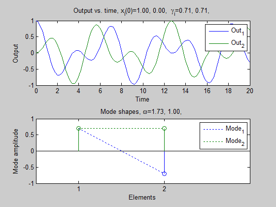
The last graph has two subplots. The top one shows the transient response of the system starting from the given initial conditions. The bottom one shows the eigenvectors (or "mode shapes") of the system. The vertical axis is magnitude, the horizontal axis is the index of the eigenvalue. The eigenvalue v1 is [0.7071; -0.7071], this is shown in blue; the first element is 0.7071 and the second element is -0.7071. The eigenvector v2 is [0.7071; 0.7071], this is shown in green. The dotted line is there simply to guide the eye (because some elements of the eigenvectors may be hidden behind another, as in the case of the first element of v1. The relevance of these shapes is discussed on the next page.
The procedure described above is easily extended to larger systems (the next page has solutions for a 3×3 and a 5×5 system). In brief:


