
Contents
While the previous pages described how to mathematically solve for the transient response of a lossless system (i.e., no friction or resistance), there was very little insight given. This page will develop physical insight into the solutions. It answers the question: "Just what do the eigenvalues and eigenvectors represent?".
The fourth order system considered here was analyzed in the example at the bottom of the previous page, and the important information is repeated here. With k1=k2=m=1, the system is defined by the fourth order matrix differential equation

The matrix A has eigenvalues and eigenvectors given by

The eigenvalues correspond to frequencies of and ω1=1.73=√3, ω2=1. The general solution of the system starting from zero velocity is given by

To determine the coefficients γ1 and γ2 we use the initial conditions (t=0) so

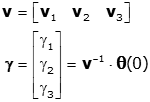
If we now define a matrix, v, whose columns are the eigenvectors we get:
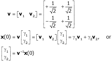
The eigenvectors determine the mode shapes, shown below.
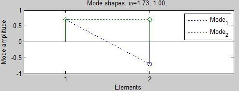
To read this graph note that

so v1 (in blue) has a height of 0.707 for the first element, and -0.707 for the second element. The other eigenvector, v2, has a height of 0.707 for both. The dotted line is there simply to guide the eye (because some elements of the eigenvectors may be hidden behind another, as in the case of the first element of v1.
Let us now try to get a deeper, more physical understanding of just what this equation represents. Let's see what happens with initial conditions

We can write
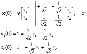
By inspection (or by solving the equation

we see that γ1=0 and γ2=√2. In this case the initial conditions were a multiple of v2, so no contribution from v1 was necessary to solve the equation

In this situation we say that mode 1 (corresponding to v1)) is not excited. Set the initial conditions in the boxes below to x1(0)=1 and x2(0)=1, then hit the "Set Initial Conditions" box and then "Start." Note: in this diagram the ends of the arrows labeled x1 and x2 correspond to the equilibrium positions of the mass (when x1=0 and x2=0)
The result is as expected. Both masses move in phase with each other. This is depicted in the mode shapes by the fact that the elements of v2 depicted are equal. This means that if only mode 2 (associated with v2) is excited, then the masses move together in phase (and the inner spring has no effect).
Now try setting the initial conditions to x1(0)=-1 and x2(0)=1 and running (hit "Set Initial Conditions" followed by "Start"). In this case the initial conditions were a multiple of v1, so only that mode was excited (γ1=-√2 and γ2=0); mode 2 is unexcited by these initial conditions. According to the mode shape, the amplitudes of the oscillations of the masses should be equal in magnitude but opposite in direction. Note that the frequency of these oscillations is higher than those associated with the second mode. This is expected mathematically (ω1=1.73=√3, ω2=1), but also physically. In mode 2, the inner spring has no effect so only the outer springs matter. In mode 1, all springs contribute so that the forces on the masses will generally be higher (for the same displacement from equilibrium), resulting in greater accelerations and faster oscillation.
If you try initial conditions close to, but not equal to, one of the modes, (e.g., x1(0)=0.8 and x2(0)=1) you will get motion that is close to that mode alone. This is because only a small contribution from the other mode is needed to meet the initial conditions.
Now try some other initial conditions (e.g., x1(0)=0 and x2(0)=1). Some complicated motions can result, but the motion is always just the linear combination of the two modes of the system.
It can be shown that the system shown
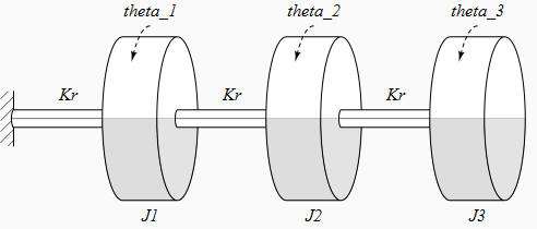
can be represented (with Kr=J1=J2=J3=1) by a fourth order matrix differential equation as

We can find eigenvalues (and associated frequencies) and eigenvectors (and associated mode shapes) using the MatLab code from the previous page. We need only change the lines defining the A matrix and the initial conditions (in this case the initial conditions themselves aren't important, but they must be in a matrix of the proper size so the code runs).
A=[-2 1 0;1 -2 1;0 1 -1];   %3 flywheels
...
x0=[1 0 0]'                 %Initial condition
The output of the code gives us the results
A matrix
    -2     1     0
     1    -2     1
     0     1    -1

Eigenvalues
   -3.2470   -1.5550   -0.1981

Eigenvectors (each column is an eigenvector)
   -0.5910   -0.7370    0.3280
    0.7370   -0.3280    0.5910
   -0.3280    0.5910    0.7370

Frequencies, omega=1.80, 1.25, 0.45,
Initial Conditions, x(0)=1.00, 0.00, 0.00,
Unknown coefficients, gamma=-0.59, -0.74, 0.33,
and the mode shapes
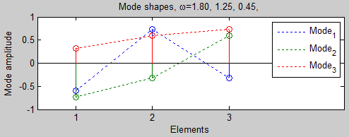
In this case there are three modes, so the general form of the solution becomes

but we can still get the unknown coefficients in the same way
As we did with the two mass system, let's try some initial conditions.
Try θ1(0)=-72, θ2(0)=90,
θ3(0)=-40
For θ1(0)=-72, θ2(0)=90,
θ3(0)=-40 we get

Clearly this set of initial conditions is very close to mode 3 (the slowest mode), and so only mode 3 is excited to any extent. You can see that (as expected from the mode shapes) the three flywheels are in phase with each other, and that J3 moves the most and J1 the least.
If you try initial conditions θ1(0)=-90, θ2(0)=-40, and θ3(0)=72, only mode 2 is excited (and the frequency is about 2.8 times faster than mode 3). The motion of J3 is out of phase by 180° from that of J1 and J2, and in this case the magnitude of the motion of J1 is greatest and J3 is least (check v3 for the exact ratios).
For initial conditions θ1(0)=-72, θ2(0)=90, θ3(0)=-40 only mode 1 is excited (and the frequency is about 4 times faster than mode 3). The motion for J2 is out of phase by 180° with that of J1 and J3, and the magnitude of J2's oscillations are greatest with J3's the smallest.
Other initial conditions (try some) result in complicated motions, but the motion can always be represents as the linear combination of the system's modes.
As with the two-mass system, the frequency of mode 3 was the slowest (ω3=0.45), followed by mode 2 (ω2=1.25) and mode 1 (ω1=1.8). We can explain this physically in the same way. For mode 3 there is very little torsion of the springs, therefore low forces, low acceleration and low frequency. For mode 1, there is the most torsion (each is out of phase with all of its neighbors). This results in high oscillation frequencies. The shape, and behavior, of mode 2 is between these.
Note: These modes are similar (but not identical) to the
first three modes of a woodwind or brass instrument (see
figure 2 at hyperlink). This is because the last element not
attached to a fixed element (like a wall) which is analogous to the open end of
a those instruments.
Now consider a system that consists of 5 masses on a string that is under uniform tension, T. Each mass, mi, has an associated position, xi, that is zero at equilibrium. The masses are equally spaced at a distance ℓ from each other.

To develop the equations of motion, consider the case when the masses are displaced from equilibrium.

Now let's examine m1 closely so we can write its equation of motion.
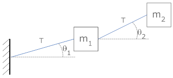
The force from each string in the vertical direction is given by the tension multiplied by the sine of the angle between the mass and the string. There is also an inertial force.
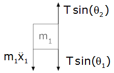
If we assume that the width of the masses as well as their vertical displacement are both small compared to the distance ℓ then we can write
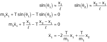
We can repeat for m2. The image shows m2 connected to m1 and m3 on the left, with a free body diagram on the right.


Likewise for m3, m4 and m5
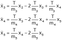
If we let m1=m2=m3=m4=m5=T=1, we get
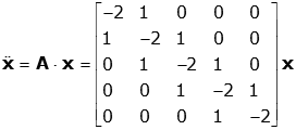
As before we can use MatLab code to get eigenvalues (and frequencies of vibration) and eigenvectors (and mode shapes). Note the A and x0 matrices in the MatLab code must be changed, as before.
A matrix
    -2     1     0     0     0
     1    -2     1     0     0
     0     1    -2     1     0
     0     0     1    -2     1
     0     0     0     1    -2

Eigenvalues
   -3.7321   -3.0000   -2.0000   -1.0000   -0.2679

Eigenvectors (each column is an eigenvector)
   -0.2887   -0.5000    0.5774    0.5000   -0.2887
    0.5000    0.5000   -0.0000    0.5000   -0.5000
   -0.5774   -0.0000   -0.5774   -0.0000   -0.5774
    0.5000   -0.5000   -0.0000   -0.5000   -0.5000
   -0.2887    0.5000    0.5774   -0.5000   -0.2887

Frequencies, omega=1.93, 1.73, 1.41, 1.00, 0.52
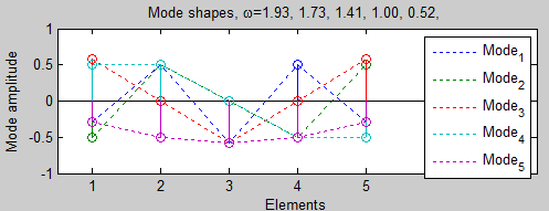
We can immediately make some comments. As before the lowest frequency mode (mode 5) has the "smoothest" shape. The shapes get increasingly oscillatory from mode 4, to mode 3, to mode 2, to mode 1; in each case, the frequency of oscillation increases.
An animation is included below. Because of the software used, the string is not shown; though it isn't shown, the system behaves as if the string was there.
Note the following:
Note: These modes are similar (but not identical) to the first five modes of a stringed instrument. This is because the both ends are fixed which is analogous to a string in a guitar or piano.