The Z Transform
Discrete Data
What is a discrete-time system and why do we care about it?
Until now we have assumed that time is continuous. In other words, time
can take on any value, and this is generally true of linear physical systems involving
components as capacitors, masses, thermal resistances... However, computers
are increasingly being integrated into systems. For the computer, time is
not continuous, it passes in discrete intervals. So whenever a computer is
being used, it is important to understand the ramifications of the inherently discrete
nature of time. As with the Laplace Transform, we will assume that functions
of interest are equal to zero for time less than zero.
Where does discrete time data come from?
Although some data associated with physical systems is inherently discrete-time
(daily high temperatures, stock closings...) most data starts out as continuous
time data and becomes discrete through a process called sampling.
For physical systems of the type considered in this course, the sampling process
is usually carried out in practice through the use of an analog-to-digital (A/D)
convertor.  The process is
often depicted as shown in the diagram at the right. In this diagram x(t)
represents a continuous-time signal that is sampled every T seconds, the resulting
signal is called x*(t). This represents a continuous-time signal that is measured
by a computer every T seconds that results in a sampled signal. A common example
of this is music stored on a CD. The continous-time signal is generated by
the human voice, pianos, guitars... and is sampled 44,100 times per second.
The resulting sequence of numbers is stored on the disc for replay at a later time .
There are a number of ways to represent the sampling process mathematically.
One way that is commonly used is to immediately represent
the sampled signal by a series x[n]. In this scheme the first sample (i.e.,
the first time the switch closes, is x[0], the next sample is x[1], and so on.
This technique has the advantage of being very simple to understand, but makes the
connection of the sampled signal to the Laplace Transform easy to understand.
We will use a different technique that is a bit more complicated mathematically
but will, in the long run, yield some physical insights not afforded by the simpler
technique. To understand the sampling process in this paradigm, first consider
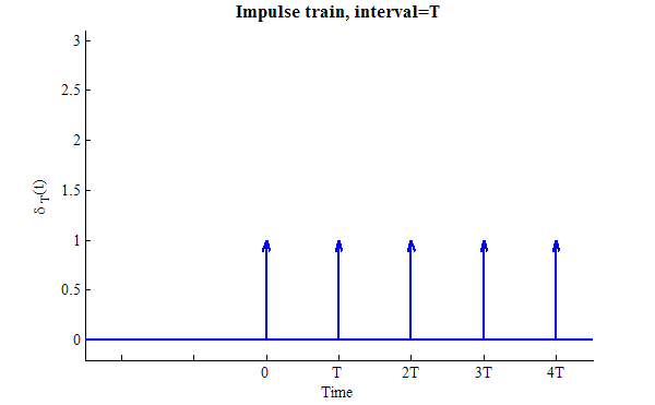
a signal that is a train of evenly spaced impulse functions. We start the
sampling function with k=0 because all of the functions that we consider will be
zero for time less than zero.

This function is shown below:
Now we can define
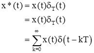
Since the product

is equal to zero except at t=kT, we can rewrite the last equation
as

This sampling process can be clarified with an image. The graph below shows
x(t),
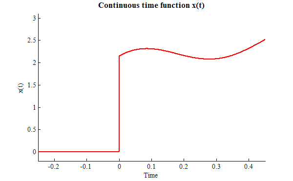
If we multiply this by the impulse train, we get the sampled function, x*(t).
For this figure, T=0.1, and the function x(t) is shown as a thin dotted red line
for reference.
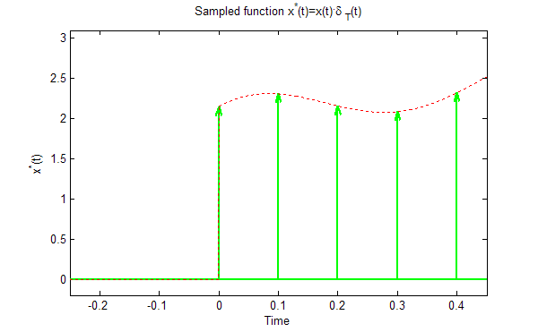
The key insight of this whole process is that the sampled function, x*(t),
is simply a train of impulses whose magnitude is given by the height of the function
x(t) (at the times x(kT)).We can rewrite the sampled signal as

where x[k] is the magnitude of the kth element in
the sequence and x[k]=x(kT). Generally when we consider a sequence we will
implicitly assume a sampling interval, T, and simply use x[k].
The Z Transform
Since we now have a time domain signal, we wish to see what kind of analysis
we can do in a transformed domain. Let's start by taking the Laplace Transform
of the sampled signal:

Since x[k] is a constant, we can (because of Linearity) bring the Laplace Transform
inside the summation.
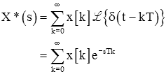
This obviously looks different than the Laplace Transforms we
have seen in the past. For one thing, there is an infinite sum. For
another, we are used to seeing functions in the Laplace domain that are the ratios
of polynomial in the variable 's,' not exponentials in 's.'
To simplify the expression a little bit, we will use the notation

so

and

We will call this the Z Transform and define it as

Key Concept: Definition of Z Transform

We say that X(z) is the Z Transform of x[k], and we can write this as

Likewise x[k] is the inverse Z Transform of X(z), or

Example: Z Transform of Finite Sequence
As a simple example, consider the sequence of sampled numbers, x[k]

For this sequence, the Z Transform of x[k] is given by:

This may seem a complicated way to define sequences, but it turns out that
many sequences of interest to us (impulse, unit step, ...) will have Z Transforms
that can be expressed in a compact form.
The Z Transform of Some Commonly Occurring Functions
This section uses a few infinite series.
The Unit Impulse Function
In discrete time systems the unit impulse is defined somewhat differently than
in continuous time systems.

The Z Transform is given by

From the definition of the impulse, every term of the summation
is zero except when k=0. So

Note that this is the same as the Laplace Transform of a unit
impulse in continuous time. The fact that the Z Transform of an impulse is
unity will yield many of the same properties, and allow for many of the same analysis
techniques (i.e., transfer functions...) to be used for discrete time systems that
were used for continuous time systems.
The Unit Step Function
The unit step is one when k is zero or positive .

The Z Transform is given by
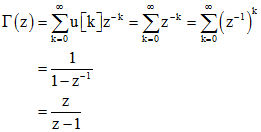
We will use the latter form, a ratio of polynomials of positive
powers of z .
The Exponential Function
Consider the exponential function:
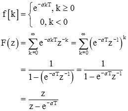
Note that this function is just the exponential function that
we are used to seeing (f(t)=e-αt, with t>0) after it has been
sampled at t=kT.
The Exponential Function Redux
With the Z Transform it is more common to get solutions in the form of a power
series:
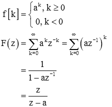
This is the same as the exponential function with a=e-αT.
Just as with continuous time systems, most of our systems will have behaviors that
consist of a sum of such exponentials.
Other Functions
The Z Transform of some other functions is given in the Table of Transforms.
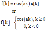
Example: Z transform of cosine
Find the Z Transform of
Solution
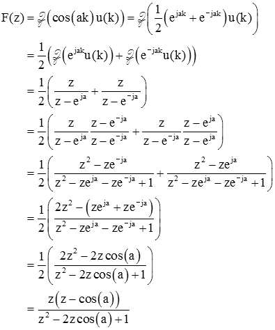
We can write

so
Some Properties of the Z Transform
As we found with the Laplace Transform, it will often be easier to work with
the Z Transform if we develop some properties of the transform itself.
Linearity
As with the Laplace Transform, the Z Transform is linear.

where

and a and b are constants.
Time Shift
An important property of the Z Transform is the time shift. To see why
this might be important consider that a discrete-time approximation to a derivative
is given by:
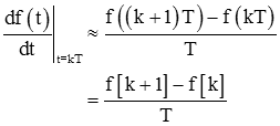
Note that this approximation involves not only t[k] but a time-shifted version
as well, f[k+1]. This is referred to as a difference equation. Let's
examine what effect such a shift has upon the Z Transform. The difference
equation will serve the same purpose with discrete time systems and the Z Transform
that differential equations served with continuous time systems and the Laplace
Transform.
Shift to the right (delay)
Consider the function x[k] shown below, which represents an arbitrary sequence.
In this figure, and subsequent figures, the samples are shown as a "stem" plot (small
circles on the end of a line).
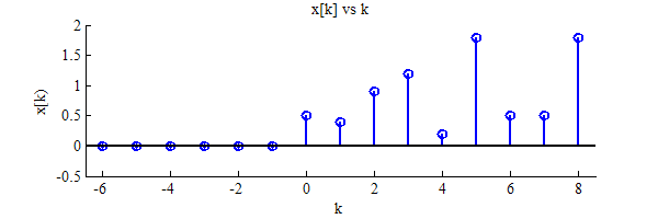
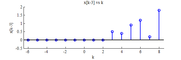
If we shift the function to the right by 3 intervals, we get the function x[k-3],
shown below.
To find the Z Transform of this shifted function, start with the definition of
the transform:

Since the first three elements (k=0, 1, 2) of the transform are zero, we can
start the summation at k=3.

Apply a change of variables
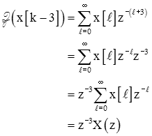
In general, a time delay of n samples, results in multiplication by z-n in the
z domain.

Shift to the left
A shift to the left is a bit more difficult. Let's explore it in the same
way as we did the shift to the right. Consider the same sequence, x[k], as
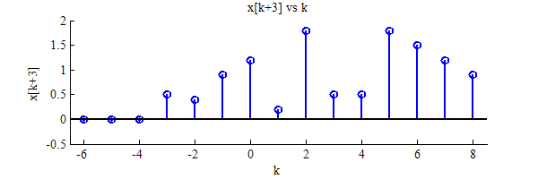
before. This time we shift it to the left by three samples to get x[k+3].
Let's try to develop the Z Transform in the same way as we did previously.
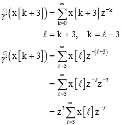
Now we run into a problem because we can't easily make the lower bound on the
summation equal to zero. However, we can add in and subtract off the first
three points, without changing the result.

Now we can combine the first two sums into one longer summation, and finish.

What we have done, in effect, is to subtract off the points that were shifted
to negative values of k (highlighted with a darker gray background below).
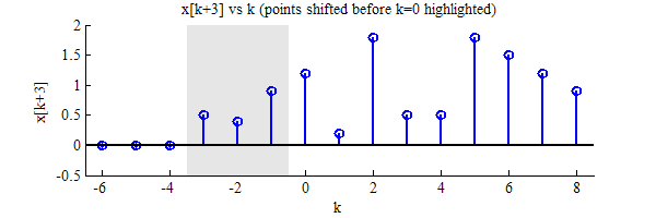
Once these points are subtracted off, we end up with a sequence that is zero
for k less than zero (below).
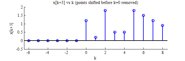
Examples: Left Shift of Z Transform
Let's consider a couple examples.
A shift of one to the left gives us:

A shift of two to the left gives us:

A shift of three gives us:

This is reminiscent of the differentiation property of the Laplace
Transform (except instead of initial conditions on the differentiated
variable with the Laplace Transform, we have initial values of the
shifted variable with the Z Transform). Each successive difference
results in a polynomial in z that is of increasingly higher order.
Key Concept: Left Shift of Z Transform
In general, for a shift to the left:

Convolution
The convolution property for the Z Transform can be proved in much the same way
as it was for the Laplace Transform. It is stated here without proof.
If y[k] is the convolution of x[k] and h[k],

then

Other Properties
These and other properties of the Z Transform are found on the Z Transform Properties table.
 Go on to the Inverse Z Transform
References
Replace
 The process is
often depicted as shown in the diagram at the right. In this diagram x(t)
represents a continuous-time signal that is sampled every T seconds, the resulting
signal is called x*(t). This represents a continuous-time signal that is measured
by a computer every T seconds that results in a sampled signal. A common example
of this is music stored on a CD. The continous-time signal is generated by
the human voice, pianos, guitars... and is sampled 44,100 times per second.
The resulting sequence of numbers is stored on the disc for replay at a later time (Note).


 Go on to the Inverse Z Transform