

For the open loop transfer function, G(s)H(s):
We have n=5 poles at s = 0,
-3 ± 2j, -2, -1. We have m=2 finite zeros at s = -1 ± 1j. So there exists
q=3 zeros as s goes to infinity (q = n-m = 5-2 = 3).
We can rewrite the open
loop transfer function as G(s)H(s)=N(s)/D(s) where N(s) is the numerator polynomial,
and D(s) is the denominator polynomial.
N(s)= s2 + 2 s + 2, and
D(s)= s5 + 9 s4 + 33 s3 + 51 s2 + 26
s.
Characteristic Equation is 1+KG(s)H(s)=0, or 1+KN(s)/D(s)=0,
or D(s)+KN(s)
= s5 + 9 s4 + 33 s3 + 51 s2 + 26 s+
K( s2 + 2 s + 2 ) = 0
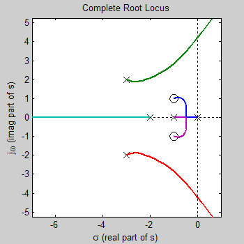
As you can see, the locus is symmetric about the real axis
The open loop transfer function, G(s)H(s), has 5 poles, therefore the locus has
5 branches. Each branch is displayed in a different color.
Root locus starts (K=0) at poles of open loop transfer function, G(s)H(s).
These are shown by an "x" on the diagram above
As K→∞ the location of closed
loop poles move to the zeros of the open loop transfer function, G(s)H(s).
Finite zeros are shown by a "o" on the diagram above. Don't forget we have
we also have q=n-m=3 zeros at infinity. (We have n=5 finite poles, and m=2
finite zeros).
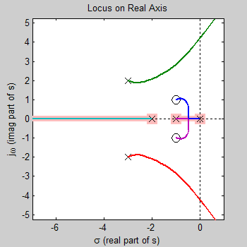
The root locus exists on real axis to left of an odd number of poles and zeros of open loop transfer function, G(s)H(s), that are on the real axis. These real pole and zero locations are highlighted on diagram, along with the portion of the locus that exists on the real axis.
Root locus exists on real axis between:
0 and -1
-2 and negative infinity
... because on the real axis, we have 3 poles at s = -1, -2, 0, and we have
no zeros.
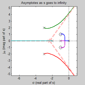
In the open loop transfer function, G(s)H(s), we have n=5 finite poles, and m=2
finite zeros, therefore we have q=n-m=3 zeros at infinity.
Angle of asymptotes
at odd multiples of ±180°/q, (i.e., ±60°, ±180°)
There exists 5 poles at
s = 0, -3 ± 2j, -2, -1, ...so sum of poles=-9.
There exists 2 zeros at s = -1 ±
1j, ...so sum of zeros=-2.
(Any imaginary components of poles and zeros cancel
when summed because they appear as complex conjugate pairs.)
Intersect of
asymptotes is at ((sum of poles)-(sum of zeros))/q = -2.33.
Intersect is at ((-9)-(-2))/3
= -7/3 = -2.33 (highlighted by five pointed star).
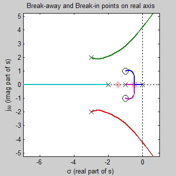
Break Out (or Break In) points occur where N(s)D'(s)-N'(s)D(s)=0, or
33 s6
+ 26 s5 + 97 s4 + 204 s3 + 274 s2 +
204 s + 52 = 0. (details below*)
This polynomial has 6 roots at s = -2.7 ±
1.1j, -0.65 ± 1.6j, -1.4, -0.46.
From these 6 roots, there exists 2 real roots
at s = -1.4, -0.46. These are highlighted on the diagram above (with squares or
diamonds.)
Not all of these roots are on the locus. Of these 2 real roots,
there exists 1 root at s = -0.46 on the locus (i.e., K>0). Break-away (or
break-in) points on the locus are shown by squares.
(Real break-away (or
break-in) with K less than 0 are shown with diamonds).
* N(s) and D(s) are
numerator and denominator polylnomials of G(s)H(s), and the tick mark, ', denotes
differentiation.
N(s) = s2 + 2 s + 2
N'(s) = 2 s + 2
D(s)= s5
+ 9 s4 + 33 s3 + 51 s2 + 26 s
D'(s)= 5 s4
+ 36 s3 + 99 s2 + 102 s + 26
N(s)D'(s)= 5 s6
+ 46 s5 + 181 s4 + 372 s3 + 428 s2 +
256 s + 52
N'(s)D(s)= 2 s6 + 20 s5 + 84 s4 +
168 s3 + 154 s2 + 52 s
N(s)D'(s)-N'(s)D(s)= 3 s6
+ 26 s5 + 97 s4 + 204 s3 + 274 s2 +
204 s + 52
Here we used N(s)D'(s)-N'(s)D(s)=0, but we could multiply by -1
and use N'(s)D(s)-N(s)D'(s)=0.
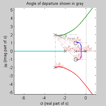
Find angle of departure from pole at -3+2j
θz1 =angle((Departing
pole)- (zero at -1+1j) ).
θz1 =angle((-3+2j) - (-1+1j)) = angle(-2+1j)
= 153.4349°
θz2 =angle((-3+2j) - (-1-1j)) = angle(-2+3j) = 123.6901°
θp1 =angle((Departing pole)- (pole at 0) ).
θp1 =angle((-3+2j)
- (0)) = angle(-3+2j) = 146.3099°
θp3 =angle((-3+2j) - (-3-2j)) =
angle(0+4j) = 90°
θp4 =angle((-3+2j) - (-2)) = angle(-1+2j) = 116.5651°
θp5 =angle((-3+2j) - (-1)) = angle(-2+2j) = 135°
Angle of Departure
is equal to:
θdepart = 180° + sum(angle to zeros) - sum(angle to poles).
θdepart = 180° + 277.125-487.875.
θdepart = -30.7°.
This angle is shown in gray. It may be hard to see if it is near 0°.
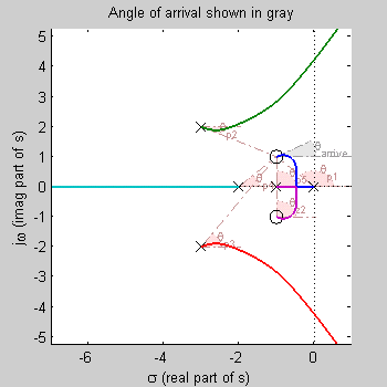
Find angle of arrival to zero at -1+1j
θz2 =angle( (Arriving
zero) - (zero at -3+2j) ).
θz2 =angle((-1+1j) - (-1-1j)) = angle(0+2j)
= 90°
θp1 =angle( (Arriving zero) - (pole at 0) ).
θp1
=angle((-1+1j) - (0)) = angle(-1+1j) = 135°
θp2 =angle((-1+1j) - (-3+2j))
= angle(2-1j) = -26.5651°
θp3 =angle((-1+1j) - (-3-2j)) = angle(2+3j)
= 56.3099°
θp4 =angle((-1+1j) - (-2)) = angle(1+1j) = 45°
θp5
=angle((-1+1j) - (-1)) = angle(0+1j) = 90°
Angle of arrival is equal to:
θarrive = 180° - sum(angle to zeros) + sum(angle to poles).
θarrive = 180° - 90 + 299.7449.
θarrive = 390°
This
is equivalent to 30°.
This angle is shown in gray. It may be hard to see
if it is near 0°.
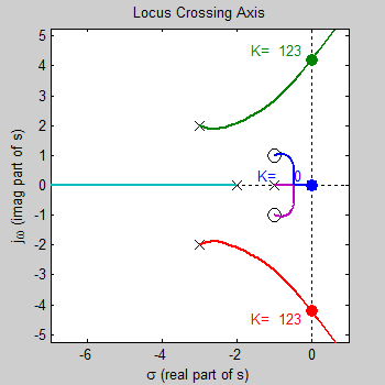
Locus crosses imaginary axis at 2 values of K. These values are normally
determined by using Routh's method. This program does it numerically, and
so is only an estimate.
Locus crosses where K = 0, 123, corresponding to
crossing imaginary axis at s=0, ±4.21j, respectively.
These crossings are
shown on plot.
Characteristic Equation is 1+KG(s)H(s)=0, or 1+KN(s)/D(s)=0,
or D(s)+KN(s)
= s5 + 9 s4 + 33 s3 + 51 s2 + 26 s+
K( s2 + 2 s + 2 ) = 0
So, by choosing K we determine the characteristic
equation whose roots are the closed loop poles.
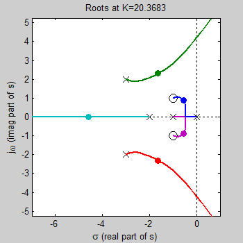
For example with K=20.3683,
then the characteristic equation is
D(s)+KN(s) = s5 + 9 s4
+ 33 s3 + 51 s2 + 26 s + 20.3683( s2 + 2 s + 2
) = 0, or
s5 + 9 s4 + 33 s3 + 71.3683 s2
+ 66.7365 s + 40.7365= 0
This equation has 5 roots at s = -4.6, -1.6 ± 2.3j,
-0.56 ±0.89j. These are shown by the large dots on the root locus plot.
Characteristic Equation is 1+KG(s)H(s)=0, or 1+KN(s)/D(s)=0, or
K = -D(s)/N(s)
= -( s5 + 9 s4 + 33 s3 + 51 s2 + 26
s ) / ( s2 + 2 s + 2 )
We can pick a value of s on the locus, and
find K=-D(s)/N(s).
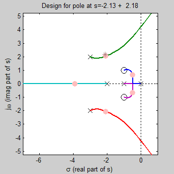
For example if we choose s= -2.1 + 2.2j (marked by asterisk),
then D(s)= 16.2 + 59.5j, N(s)=-2.46 + -4.91j,
and K=-D(s)/N(s)= 11 + 2.21j.
This s value is not exactly on the locus, so K is complex, (see note below), pick
real part of K ( 11)
For this K there exist 5 closed loop poles at s = -3.9,
-2.1 ±2j, -0.48 ±0.66j. These poles are highlighted on the diagram with dots,
the value of "s" that was originally specified is shown by an asterisk.
Note:
it is often difficult to choose a value of s that is precisely on the locus, but
we can pick a point that is close. If the value is not exactly on the
locus, then the calculated value of K will be complex instead of real. Just ignore
the the imaginary part of K (which will be small).
Note also that only one
pole location was chosen and this determines the value of K. If the system has more
than one closed loop pole, the location of the other poles are determine solely
by K, and may be in undesirable locations.