BodePlotGui: A Tool for Generating Asymptotic Bode Diagrams
BodePlotGui is a
graphical user interface written in the MATLAB® programming language. It
takes a transfer function and splits it into its constituent elements, then
draws the piecewise linear asymptotic approximation for each element. It
is hoped that the BodePlotGui program will be a versatile program for teaching and learning the construction of Bode diagrams from piecewise linear approximations.
Files for the program
are found here.
Note: the MATLAB GUI doesn't display well on all devices (some elements of the GUI may not show up). If you have this problem, simply run the MATLAB command "guide" and open the fileBodePlotGui.fig. You can edit the size and layout of the GUI for your machine. Save it, and then rerun the BodePlotGui.m file.
I have stopped working on BodePlotGui and have developed a similar tool in JavaScript to make it more accessible (see the "Drawing Tool" tab, above). While MATLAB is extremely powerful, it is also very expensive.
Use of program.
A Simple Example.
Consider the transfer function:

This function has three terms to be considered when constructing a Bode diagram, a constant (100), a pole at ω=10
rad/sec, and a zero at the origin. The following MATLAB® commands begin execution of the GUI:
>>MySys=tf(1000*[1 0],[1 10]);   %define Xfer function
>>BodePlotGui(MySys)        %Invoke GUI
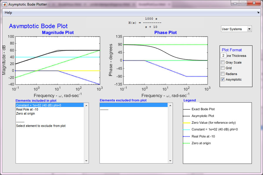
The GUI generates a window as shown
below.

Starting in the upper left and going
counterclockwise, the windows show:
- The magnitude plot, both the piecewise linear approximation for all three terms as well as the
asymptotic plot for the complete transfer function and the exact Bode diagram for magnitude. Also shown is a zero reference
line.
- The phase plot.
- A list of the systems in the user workspace.
- Several checkboxes that let the user format the image. In
particular there is a check-box that determines whether or not to
display the asymptotic plot for the complete transfer function;
sometimes it gets in the way of seeing the other plots, so you may
want to hide it.
- The legend identifying individual terms on the plot.
- A box that shows elements excluded from the plot. This box is empty in this display because the diagram displays all three elements of the transfer function.
- A 'Legend' box that shows elements displayed in the plot.
- Several
check-boxes that allow the user to display how the plots are
displayed
- Also in the upper left is a "Help" tab.
Also shown in the upper right hand corner is the transfer function, H(s).
Modifying what is displayed
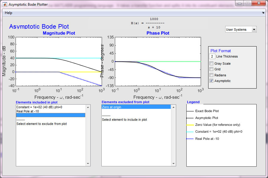
The function displayed can be manipulated term by term to illustrate the effect of each term. For example, the zero at the origin can be excluded simply by clicking on it in the lower left hand box.
The figure below shows the result.

Note that the zero
at the origin is no longer included in the plot. Each term can be
likewise included or excluded by simply clicking on it.
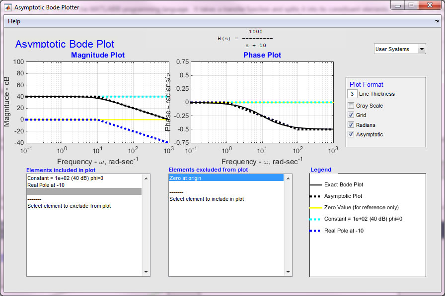
The next plot shows
the plot modified to have thicker lines, a grid, phase in radians and
with the asymptotic plot of the complete transfer function. In the
previous graph, the phase of the asymptotic plot obscured that of the real
pole; this is an example when it might be convenient not to show the asymptotic
approximation.

Underdamped terms
Underdamped poles
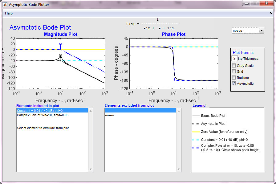
(and zeros) present a difficulty because they cause a peak (dip) in the
magnitude plot. The program show this with a simple circle showing the
peak height. For example the transfer function

yields the output
shown below. The peak due to the underdamped pole is clearly shown.

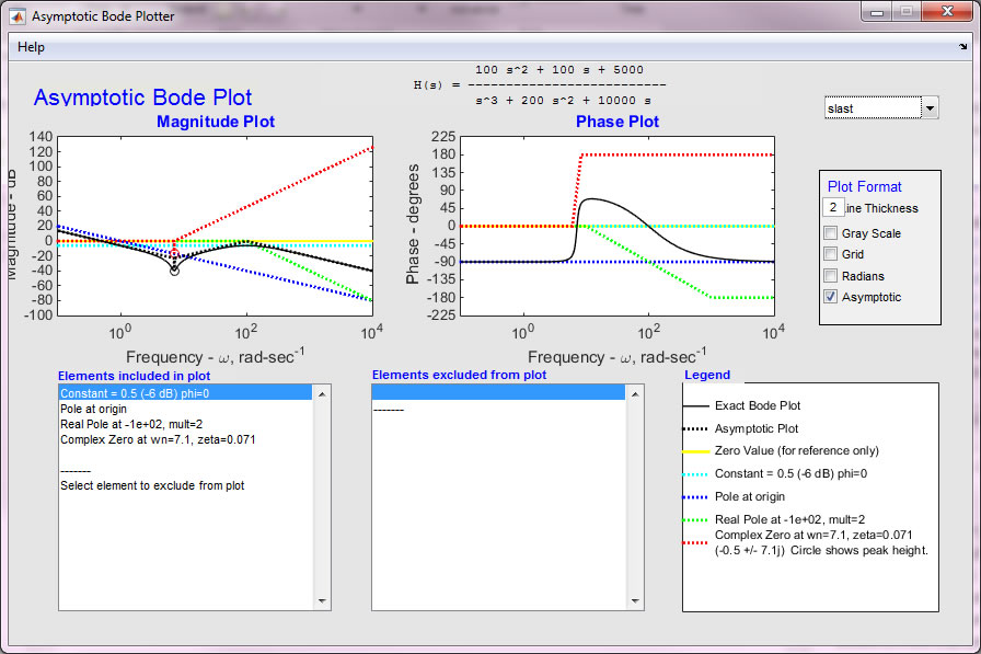
A more complicated example
The example below is
more complicated. It shows underdamped terms, repeated poles, and a
pole at the origin.


Limitations of the software:
The software has known limitations. It does not calculate the phase associate with a time delay. It only decomposes transfer functions with up to
20 separate terms (a limit only of the number of colors used). Repeated poles and zeros are treated as a single term (i.e., it is not possible to move only one pole of a repeated pair from the “Elements included in plot” window to the “Elements excluded from plot” window of the GUI).
→Get the files
→
References
Replace

