
Contents
A time delay is common in the study of linear systems. For example, a car running over a curb can be modeled as a step up at time=0 (as it hits the curb) followed by a step down that is delayed (as it comes off the curb on the other side). A substance injected at one end of a pipe with liquid flowing appears at the other end after a time delay. The list is endless.
This document explores the expression of the time delay in the Laplace domain. We start with the "Time delay property" of the Laplace Transform:

which states that the Laplace Transform of a time delayed function is Laplace Transform of the function multiplied by e-as, where a is the time delay. We commonly explore systems as a function of frequency (e.g., Bode plots). Let's examine what the time delay looks like as a function of frequency.
To examine the frequency domain representation of the time we let s=jω.

In the frequency domain, we are concerned with two quantities, the magnitude and the phase. The magnitude of the time delay in the frequency domain is

This tells us that the magnitude of a time delay is just unity, and is independent of frequency. This makes sense - if you delay a signal, you are not changing the magnitude of the signal, you are only changing the timing of the signal. Therefore we expect that the phase associated with a time delay will not be constant:

The phase shift associated with a time delay decreases linearly with a slope of -ωa, where a is the length of the time delay.
If we examine the time delay in the frequency domain, we do so with plots of
magnitude and phase. Shown below are linear plots of magnitude and phase
for a time delay of 2.5 seconds, plotted on a linear scale vs. frequency.
Frequency goes from 0.1 to 100 radians per second. You can see that the
magnitude is constant at one, and the phase drops linearly with a slope of -2.5.
(Note: at ω=2·π rad/sec, φ (in radians) = -ω·a = -2·πrad/sec·2.5sec =
-15.71 rad.)
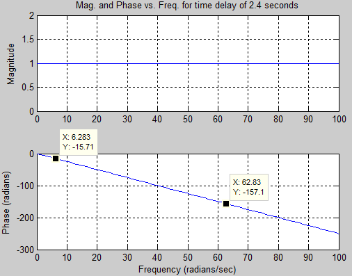
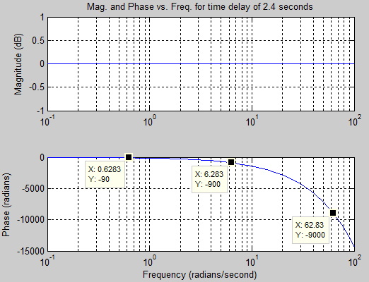
Magnitude and phase are more commonly plotted in Bode plots as deciBel
magnitude, phase as degrees, and using a logarithmic frequency scale. The
phase plot, in particular, looks very different. Because the phase drops
linearly, but the scale is logarithmic, the phase plot actually drops
exponentially (e.g., the frequency 0.2·π, 2·π and 20·π are equally spaced on the plot, but the corresponding frequencies are -90, -900, and -9000°;
i.e.,
decreasing exponentially.)
(Note: at ω=2·π rad/sec, φ(in degrees) = -ω·a·180/(2*π)
= -2·π·rad/sec·2.5sec·180/(2·π) = -900°)
To understand why the phase shift associated with a time delay is linearly proportional to the phase of the signal consider three sine waves (at 100, 200 and 400 Hz) each delayed by 1.25 mSec.
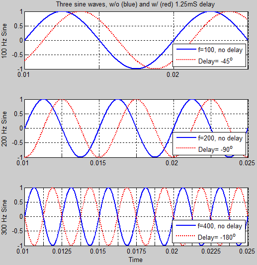
You can see from the graphs, that the phase shift associated with a delay of 1.25 mS is
Because the time delay cannot be expressed as a ratio of polynomials, systems with time delays are not amenable to solution by some standard methods (root locus, routh-horwitz...). However, we can approximate the delays in terms of various polynomial expansions.
The most obvious polynomial expansion of the exponential is the Taylor series

As an example a second order approximation of a 2 second time delay yields

This technique is extremely limited because the order of the numerator is greater than the order of the denominator and many of our techniques are limited to systems for which the order of the numerator is equal to or less than that of the numerator.
However we can develop an approximation that consists only of poles by putting the exponential term in the denominator:

A second order approximation of a 2 second time delay yields

The graph below shows the step response of a pure two second time delay along with a 1st, 2nd and 3rd order expansion.
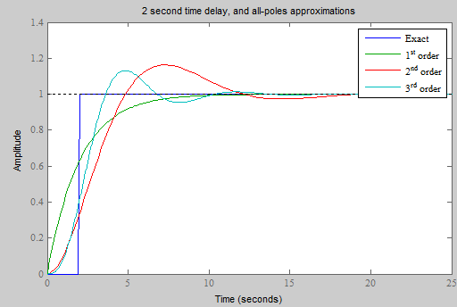
You can see that as the order of the approximation increases, the approximation improves (but so does the complexity).
An even better method of approximating the exponential uses "Padé" approximation (see wikipedia page, and Matlab help ("doc pade")). The Padé approximation is expressed as a ratio of polynomials. The first three Padé approximations to the time delay are:
| 1st order |
 |
| 2nd order |
 |
| 3rd order |
 |
The graph below shows the step response of a pure two second time delay along with a 1st, 2nd and 3rd order Padé approximations.
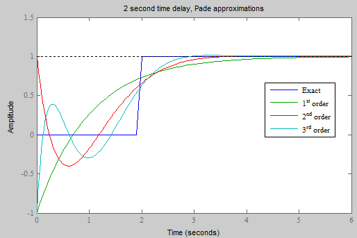
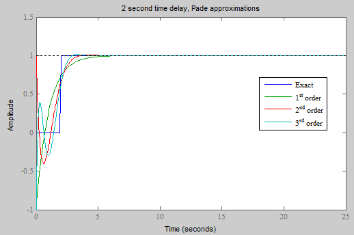
If we show the graphs on the same time scale as the "All poles" approximation, you can see that the Padé works much better (less overshoot, faster convergence...), though they have larger excursions from the exact response at small times.
© Copyright 2005 to 2019 Erik Cheever This page may be freely used for educational purposes.
Erik Cheever Department of Engineering Swarthmore College