Matlab for Laplace Transform Inversion / Partial Fraction Expansion
Contents
The code that generated this page is available at: http://lpsa.swarthmore.edu/LaplaceXform/InvLaplace/PFE1Matlab/PFE1.m
Background: Matlab and polynomials
Define the polynomial 
F=[1 3 2]
F = 1 3 2
Display it
poly2str(F,'s')
ans = s^2 + 3 s + 2
Evaluate it as s=1
polyval(F,1)
ans = 6
Find roots, Note that since roots are at -1 and -2 the polynomial is (s+1)(s+2)
roots(F)
ans =
    -2
    -1
Define a second polynomial by its roots The polynomial is 
G=poly([-1+2j -1-2j -1 0 0]);
poly2str(G,'s')
ans = s^5 + 3 s^4 + 7 s^3 + 5 s^2
Multiply polynomials H=FG (use convolution command)
H=conv(F,G)
H = 1 6 18 32 29 10 0 0
First Example - Simplest case - distinct real roots
To see this example worked out manually go to: http://lpsa.swarthmore.edu/LaplaceXform/InvLaplace/InvLaplaceXformPFE.html#Distinct_Real_Roots_
disp('Example 1: PFE with distinct real roots');
Example 1: PFE with distinct real roots
This case considers only distinct real roots.

Define numerator and denominator polynomial.
n=[1 1];                %n=s+1
d=conv([1 0],[1 2]);    %Use "conv" to multiply polynomial
disp(['Numerator = ' poly2str(n,'s')]);
disp(['Denominator = ' poly2str(d,'s')]);
Numerator =    s + 1
Denominator =    s^2 + 2 s
Now use "residue" command to do inverse transform. r = magnitude of expansion term p = location of pole of each term k = constnat term (k=0 except when numerator and denominator are same order (m=n)).
[r,p,k]=residue(n,d)
r =
    0.5000
    0.5000
p =
    -2
     0
k =     []

Note that the function is implicitly defined only for t>=0. Some texts show the time domain function multiplied by the unit step. We will keep our expressions simpler by making that relationship implicit.
Second Example - Repeated roots at origin
To see this example worked out manually go to: http://lpsa.swarthmore.edu/LaplaceXform/InvLaplace/InvLaplaceXformPFE.html#Repeated_Real_Roots_
disp('Example 2: PFE with repeated real roots (at origin in this case)');
Example 2: PFE with repeated real roots (at origin in this case)

Define numerator and denominator polynomial.
n=[1 0 1];    %n=s^2+1
d=[1 2 0 0];  %d=s^2(s+2)=s^3+2s^2
disp(['Numerator = ' poly2str(n,'s')]);
disp(['Denominator = ' poly2str(d,'s')]);

[r,p,k]=residue(n,d)
Numerator =    s^2 + 1
Denominator =    s^3 + 2 s^2

r =
    1.2500
   -0.2500
    0.5000
p =
    -2
     0
     0
k =     []
Note, first order term (1/s) comes before the 2nd order term (1/s^2) in the Matlab results.


Third Example - Complex Conjugate roots
To see this example worked out manually go to: http://lpsa.swarthmore.edu/LaplaceXform/InvLaplace/InvLaplaceXformPFE.html#ExampleRepeat
disp('Example 3: PFE with complex conjugate roots.');
Example 3: PFE with complex conjugate roots.

Define numerator and denominator polynomial.
n=[5 8 -5];     %n=s^2+1
d=[1 2 5 0 0];  %d=s^2(s^2+2s+5)=s^4+2s^3+5s^2
disp(['Numerator = ' poly2str(n,'s')]);
disp(['Denominator = ' poly2str(d,'s')]);

[r,p,k]=residue(n,d)
Numerator =    5 s^2 + 8 s - 5
Denominator =    s^4 + 2 s^3 + 5 s^2

r =
  -1.0000 - 1.0000i
  -1.0000 + 1.0000i
   2.0000 + 0.0000i
  -1.0000 + 0.0000i
p =
  -1.0000 + 2.0000i
  -1.0000 - 2.0000i
   0.0000 + 0.0000i
   0.0000 + 0.0000i
k =     []
Note, first two roots are complex conjugate roots.
Get magnitude and phase from magnitude and phase of pfe Refer to manual solution on web page listed above.
M=2*abs(r(1))       %Magnitude of cosine
phi=angle(r(1))     %Phase of cosine in radians
M =    2.8284
phi =   -2.3562
Get frequency and decay rate from location of pole
omega=abs(imag(p(1)))   % omega has to be positive
alpha=-real(p(1))
omega =     2
alpha =     1

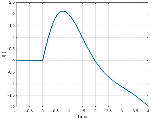
Plot the response
t=linspace(-1,4,1000);
f=(M*exp(-alpha*t).*cos(omega*t+phi) + r(3) + r(4)*t) .* heaviside(t);
plot(t,f,'Linewidth',2);
xlabel('Time'); ylabel('f(t)'); grid;

Fourth Example - Order of numerator=order of denominator
To see this example worked out manually go to: http://lpsa.swarthmore.edu/LaplaceXform/InvLaplace/InvLaplaceXformPFE.html#Order_of_numerator_polynomial_equals_order_of_denominator_
disp('Example 4: PFE: order of num=order of den');
Example 4: PFE: order of num=order of den
If the numerator and denominator have the same order, we get a constant as part of the partial fraction expansion.

Define numerator and denominator polynomial.
n=[3 2 3];          %n=3s^2+2s + 3
d=[1 3 2];          %d=s^2+3s+2=(s+1)(s+2)
disp(['Numerator = ' poly2str(n,'s')]);
disp(['Denominator = ' poly2str(d,'s')]);

[r,p,k]=residue(n,d)
Numerator =    3 s^2 + 2 s + 3
Denominator =    s^2 + 3 s + 2

r =
   -11
     4
p =
    -2
    -1
k =     3
Note this time that k is not empty, k=3.

