Drawing the asymptotic diagrams for underdamped second order systems is more involved than for first order systems. This document describes in details a few different choices for asymptotic magnitude and phase approximations for underdamped systems.
Magnitude plots for underdamped second order systems are difficult and there is no obvious way to do so. This document presents two methods, either of which is appropriate. The Matlab code used to generate the plots is here.
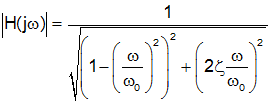
The magnitude due to a second order underdamped pair of poles is given by

It can be shown that a peak occurs in the magnitude plot near the break frequency. The exact height and location can be determined by differentiating the expression for the magnitude of the transfer function with respect to frequency and setting it to zero (to make life easier, square the function before differentiating, since the peak will be in the same place for a function or its square). The resulting differentiation shows a peak at the frequency given by

By putting this expression for ωr into the expression for |H(jω)| above, it can be shown that

Note that the peak only exists for 0<ζ<0.707=1/√2 and the frequency of the peak is typically very near the break frequency. For ζ=0, the peak is exactly at the natrual frequency (ω0) but the peak frequency drops as ζ increases.
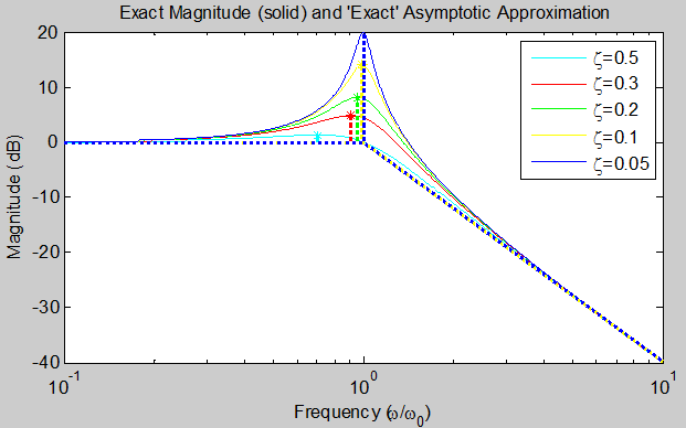
To draw a piecewise linear approximation, use the low frequency asymptote up to the break frequency, and the high frequency asymptote thereafter. Add a peak at the resonant frequency, ωr, given by

with amplitude given by

You can then draw a smooth curve between the low and high frequency asymptote that goes through the peak value.
The graph below shows this method applied to underdamped systems with several value of ζ.
The method discussed above finds the exact resonant frequency and peak height and uses them to create the asymptotic approximation. However, when sketching by hand, it is often useful to favor speed over precision (if precision is necessary, it is better to use a tool like Matlab to make the plot). For example, the exact resonant frequency is given by

However, as the table below shows, even for a fairly large ζ of 0.3 (which has a small peak of only 5 dB), the resonant frequency only shows a 9.1% deviation from the break frequency. Hence when we make the asymptotic approximation we will put the peak at the break frequency rather than the true resonant frequency, (i.e., we assume ωr≈ω0).
| ζ | Peak frequency | Peak Height | |||||
| Exact | Approx | % diff | Exact | Approx | % diff | ||
 |
 |
 |
 |
||||
| 0.5 | 0.71ω0 | ω0 | 29% | 1.15 | 1.00 | 15% | |
| 0.4 | 0.83ω0 | ω0 | 17% | 1.37 | 1.25 | 9.1% | |
| 0.3 | 0.91ω0 | ω0 | 9.5% | 1.75 | 1.67 | 4.8% | |
| 0.2 | 0.96ω0 | ω0 | 4.1% | 2.55 | 2.50 | 2.1% | |
| 0.1 | 0.99ω0 | ω0 | 1.0% | 5.02 | 5.00 | 0.5% | |
| 0.05 | 1.00ω0 | ω0 | 0.3% | 10.0 | 10.0 | 0.1% | |
Note: though some of the errors on this chart seem large, recall that both frequency and peak height are plotted on a logarithmic scale which tends to minimize differences.
We can also make an approximation for the magnitude of the resonant peak. The exact expression for the peak amplitue is

However, if ζ is less than 1, then ζ2 is even smaller. If we subtract from 1 we get a number near 1. When we take the square root of a number near 1, the result is even closer to 1. So we will use the approximation

and

Again, consulting the table above we see that we get a deviation of only 4.8% when ζ=0.3.
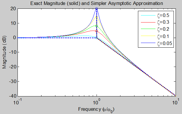
To draw a piecewise linear approximation, use the low frequency asymptote up to the break frequency, and the high frequency asymptote thereafter. Add a peak at the break frequency, ω0, with amplitude given by

You can then draw a smooth curve between the low and high frequency asymptote that goes through the peak value.
The graph below shows this method applied to underdamped systems with several value of ζ. While not quite as accurate as the "exact" method described previously, it is close enough to use for sketching by hand.
Phase plots for underdamped second order systems are difficult and there is no obvious way to do so. This document presents three methods, any of which is appropriate. The Matlab code used to generate the plots is here.
This approximation was developed by trial and error to try to minimize the maximum error between the asymptotic phase diagram and the exact phase diagram. For the asymptotic approximation to the phase of a second order pole we draw a line from 0° at

to -180° at

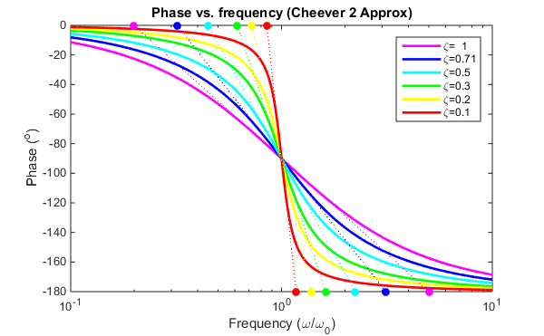
This approximation, along with the exact phase diagram, is shown below for several values of ζ
This method relies on matching the slope of the phase at the break frequency (since we know the break frequency, if we also know the slope, we can draw an asymptotic approximation). The phase as a function of frequency is given by:
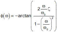
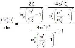
The slope of the phase is (using Matlab's symbolic toolbox)
This can be simplified to:
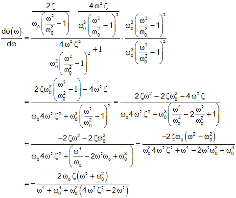
If we evaluate this at the break frequency we get

We also know that the phase looks like a straight line on the semilog plot of phase vs. frequency near ω=ω0. We can express the straight line approximation by:

(Note: this goes through π/2 at
ω=ω0, and is a straight line on a semilog plot)
We now find the slope of the straight line approximation

and equate it to the previously calculated slope of the phase at ω=ω0, and solve for the quantity "m."
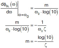
This gives us our straight line approximation for the angle:

To form the asymptotic approximation we want to know the frequency at which the straight line approximation goes to 0° (call this ωlow) and when the approximation goes to -180°, or -πrad (call this ωhigh).
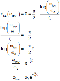
We can use the approximation

to simplify even further.

By a similar set of calculations we get

For the asymptotic approximation to the phase of a second order pole we draw a line from 0° at

to -180° at

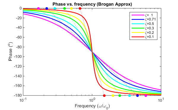
Brogan has developed another approximation. For the asymptotic approximation to the phase of a second order pole we draw a line from 0° at

to -180° at

This approximation, along with the exact phase diagram, is shown below for several values of ζ
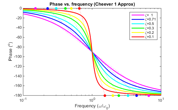
The method we will use is an extension of the one used for first order poles. In particular, for a first order pole with a break frequency at ω0 the phase plot is at 0° until ω0/10 and then rises linearly to +90° at 10·ω0. For a second order pole we change this to: the phase plot is at 0° until ω0/10ζ (or ω0·10-ζ) and then drops linearly to -180° at 10ζ·ω0. Note that for ζ=1 (critical damping) this becomes the same as the rule for a single real pole. This approximation, along with the exact phase diagram, is shown below for several values of ζ.
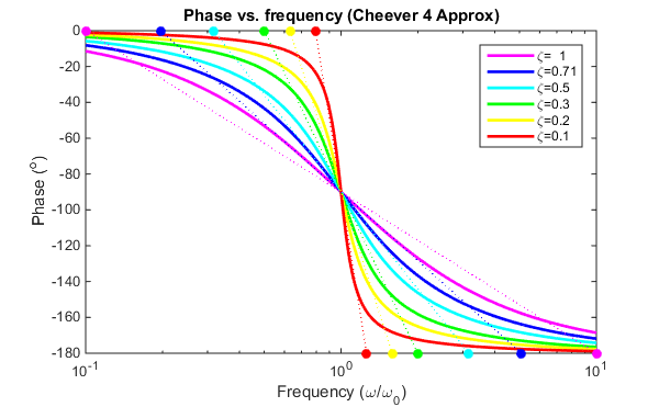
In comparison with method 2 (matching the phase of the slope at ω=ω0), this method is less accurate near ω0, but is a better overall approximation and has lower maximum error as is seen in the graph below that compares the two methods for ζ=0.5.
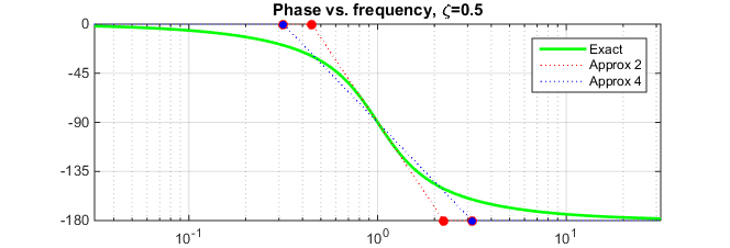
However it has the advantage of being very easy to plot on semilog paper. Since the number 10·ω0 moves up by a full decade from ω0, the number 10ζ·ω0 will be a fraction ζ of a decade above ω0. On the graph above you can see that the corner frequencies for ζ=0.5 fall midway between ω0 and ω0/10 (at the lower break frequency) to midway between ω0 and ω0·10 (at the higher frequency).